Chapter 6 Hypothesis Testing
6.1 Descriptive and Inferential Statistics
Statistics is a tool to clarify our observations of variability. This is the first function of statistics, descriptive statistics. Descriptive statistics offers a number of tools to describe variability. Descriptive statistics is useful because we can understand variability better with statistics better than we can intuitively. Imagine the challenge of summarizing hundreds of scores simply by looking at the values. Reporting the mean can tell us a lot about many scores by summarizing them with one number. This is the purpose of descriptive statistics, to summarize distributions of scores.
Inferential statistics is the process of drawing conclusions about the variability of a group of interest (called a population) using a limited set of data (called a sample). Fundamentally, inferential statistics use probability theory and logic that allow you to make conclusions about populations. This process is called null hypothesis significance testing (NHST).
Example: I am interested in middle school students’ reading comprehension in the United States, and I want to see if it changes over time. To understand this population directly, I would have to measure the reading comprehension of every member. This is impossible. Instead, I take a random sample from the population by mailing surveys to 50 random middle school students with consent of their parents, I can use descriptive statistics to understand my sample data (50 scores) and inferential statistics to generalize the results to the population (thousands of scores).
6.2 Null Hypothesis Significance Testing (NHST)
We won’t be doing statistical analysis by hand in this class. Rather, it’s more important that you understand how null hypothesis significance testing (NHST) works, because it is part of every inferential statistical analysis. We will use a two-sample t-test as an example. Let’s imagine we want to improve the reading comprehension of middle schoolers, and we have an experiment set up to do so. We developed an afterschool program for middle schoolers. We created two randomly-assigned groups, one receiving the afterschool program and the other participating in a physical education afterschool program (to serve as our control). After six weeks of the program, all participants take a reading comprehension test, which is scored as percentage correct (from 0% to 100%). You’ll notice we have a discrete, dichotomous IV and a continuous, quantitative DV; excellent variables for a t-test.
NHST sets up two competing hypotheses. In fact, they are opposites of each other. NHST hypotheses are not the same thing as the research hypothesis that we have discussed previously. NHST hypotheses are used only for running a statistical analysis. In NHST, you are trying to prove that one of the two hypotheses, the null hypothesis, is false. You start by setting up your two hypotheses (hypotheses is the plural of hypothesis):
- The null hypothesis (symbol is \(H_0\)). The null hypothesis is the hypothesis of no effect. The null hypothesis is what we would expect to happen if there was no manipulation, or if our manipulation did not do what we expected (i.e., the manipulation has no effect). It is the opposite of the hypothesis you want to demonstrate. In our example, the null hypothesis is that “students in the afterschool program will not have a higher reading comprehension, on average, than students in the physical education group.”
- The alternative hypothesis (symbol is either \(H_1\) or \(H_a\)). is the hypothesis that there is an effect. In our example, the null hypothesis is that “students in the afterschool program will have a higher reading comprehension, on average, than students in the physical education group.” The alternative hypothesis is what you ultimately want to demonstrate; it is usually similar to your research hypothesis for the study. You demonstrate the alternative hypothesis by demonstrating that the data you obtained are unlikely if the null hypothesis was true. That’s a complex sentence we will unpack further, but when you understand the previous sentence, you are on your way to mastering NHST.
These are the steps in the process:
- Assume the null is true. We assume the null hypothesis to be true. We are setting up a demonstration that says, “okay, if you are skeptical that my afterschool program is effective, let’s see how likely it is that student scores could go up with me doing nothing.”
- How could this happen? Scores fluctuate due to sampling error. Sampling error is variation due to who ends up being selected for the sample. Every time we take a random sample from a population, we don’t get the exact same mean.
- In NHST, we will find out how likely it is that we could get these results because of sampling error.
- Imagine that your afterschool group scored 0.05% higher on the reading test than the control group. Do you think it’s likely or unlikely that sampling error was the reason for the increase? Do you think it’s likely that the afterschool program raises reading scores?
- Now imagine that your afterschool group scored 35% higher on the reading test than the control group. Do you think it’s likely or unlikely that sampling error was the reason for the increase? Do you think it’s likely that the afterschool program raises reading scores?
- Later, we will calculate the likelihood that the difference is due to sampling error (that is, random chance). The name for this calculation is p.
Set the alpha level. We set a threshold for how much evidence we need (how low of a p-value we need). We call this the alpha level. By convention, we set alpha to .05 (5%). Assuming the null hypothesis is true, this means a 5% chance of results being due to sampling error.
Write null and alternative hypotheses. Write hypotheses (singular: hypothesis). Write the formal hypotheses, an \(H_0\) and an \(H_a\). The alternative hypothesis is what we aim to demonstrate. We proceed to the next step continuing to assume the null hypothesis is true.
Null hypothesis: Students in the afterschool program will not have a higher reading comprehension, on average, than students in the physical education group.
Alternative hypothesis: Students in the afterschool program will have a higher reading comprehension, on average, than students in the physical education group.
Analysis. In this step, we compute a statistic from our sample data. A statistic is anything that Here, our statistic is t, which measures the mean difference between our two groups. If the two groups have similar reading scores, the value of t will be near zero. If the two groups have different reading scores, the value of t will move away from zero (either negatively or positively). SPSS will also compute p, the probability that you could have obtained this statistic by chance if the null hypothesis were true. p is based on two things: the statistic (in this case, t) and sample size (n). Another way to understand p: If the null were true (there was no effect to find) and we ran our study 100 times with 100 different samples, how many of those samples would have a value of t at least as large as the one we obtained?
Decide to reject or retain. Decide if the statistic is in the critical region . In other words, decide if your observed statistic is likely (p > .05) or unlikely (p < .05) to have occurred if the null hypothesis were true. If p < .05, you reject the null hypothesis. If p > .05, you retain the null hypothesis.
Conclude or no conclusions. If you reject the null, your conclusion is that you have evidence for the alternative hypothesis. Important: If you end up retaining the null hypothesis (i.e., you did not find an effect), then you can make no conclusion statements—Your research has demonstrated nothing.
6.3 NHST Can Be Confusing
NHST confuses many students. It’s counterintuitive! Please come to class with your questions.
Students are not the only ones confused. NHST confuses scientists, as well. Some common misunderstandings about NHST:
p is not probability of the null being false. Since we really want to know if the null is true or false, it’s natural to think that p provides this information, but it does not. p is the probability of obtaining a sample statistic at least this extreme, assuming the null is true.
p is based on conditional probability, which confuses many people. p is a probability that already assumes the null hypothesis is true. Any statement about p should begin with “Assuming the null is true…”. People fall into the trap of reversing the conditional probability when they think p is the probability of a hypothesis. Assuming I start with a brand-new deck of cards, what is the probability of drawing red? It’s 50%. Let’s reverse the conditional probability: Assuming I drew a red card from a second deck, what is the probability of the second deck being new? It’s not 50%; the probability of red depends on the deck being new, but the probability of the deck being new does not depend on drawing a red card. We make same mistake with NHST. P is probability of obtaining these data if the null were true. It is not the probability of the null being true if we obtained these data.
Your decision to retain or reject is all-or-nothing. You either reject or retain. There is no grey area. There is no such thing as “highly significant” or “approaching significance.” These lead to misunderstandings of NHST.
Affirming the null is a tempting logical fallacy. Affirming the null is when a non-significant effect is taken as evidence of something. If the results of your drug trial are non-significant, you have not shown that your experimental drug has no effect. Rather, you have shown nothing; your results are inconclusive. Only rejecting the null allows conclusions to be made. For this reason, avoid the term “insignificant.” Instead, use “not significant” or “did not reach significance.”
Just because a result is significant does not mean it is important. For example, would you invest in an insomnia drug that has been shown to help people sleep for one additional minute per night, on average? NHST helps you decide but going back to the data is needed to interpret the real-world meaning of your results.
6.4 Conducting an Independent Samples t-Test
To simplify the procedure, we are only doing an independent samples t-test for now. Additionally, we will focus on obtaining and interpreting the p-value and mean difference. We are skipping assumption checks and conducting all of these as two-tailed tests.
6.4.1 Analyze & Decide – Using SPSS
- Select “Independent-Samples T Test.”
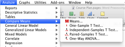
SPSS Analyze menu showing Compare Means selected
- Move the dependent variable into the “Test Variable(s)” box. Move the grouping variable into the “grouping variable” box.
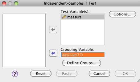
SPSS Independent-samples t test dialog box
- Click “Define groups” and then set the button to “Use specified values.” You have to tell SPSS what your coding scheme is for the grouping variable. In this example, our groups are “1” and “2”. Click “Continue.”
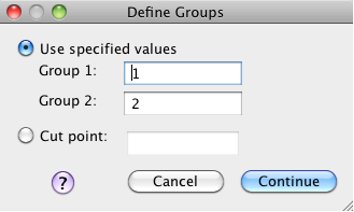
SPSS Define Groups dialog box
- Click “OK.”
Look for the “Sig. (2-tailed)” column (note: this is the one near the middle of the table–be careful so that you don’t accidentally use the Levine’s test Sig. value). For now, find the value in the “equal variances assumed” row. In SPSS, Sig. means ‘p’. This is the p value of your test.
Decide: If p is less than .05, then you reject the null hypothesis (there is a significant difference between the groups). If p is greater than or equal to .05, retain the null hypothesis (no conclusions can be made).

SPSS independent samples t-test output