Chapter 17 One Variable and Two Variable Chi-Square
17.1 Nonparametric tests
Chi-square is a nonparametric test. All other tests we have seen in the course have been parametric tests. That is, they make assumptions about the populations from which the samples are drawn. Nonparamteric tests, chi-square included, make minimal assumptions about the underlying populations.
The problem chi-square solves is the problem that comes up when you have a qualitative DV. We have used qualitative data (nominal and ordinal data) as an IV throughout the course. Now, we can use qualitative data as a DV.
For example, imagine you are doing research to see if subliminal messages affect whether people perceive a word as emotionally positive, negative or neutral. Participants respond to words with one of these three labels. Because this data is qualitative, the emotionality of the word cannot be a DV in an ANOVA or multiple regression. With a one-sample chi-square test (also called the chi-square test for goodness-of-fit), you can use emotionality as a DV.
Nonparametric tests carry fewer assumptions. There are still some assumptions, however. Sampling still needs to be random, and observations are assumed to be independent.
There is a cost for using a test with fewer assumptions. The cost is power. In data where the null hypothesis is truly false, a nonparametric test has a lower chance of rejecting the null hypothesis than its parametric version.
In short, use nonparametric tests when you need to. One reason you need to use nonparametrics tests is if you have a qualitative DV.
17.2 Two kinds of chi-square tests
There are two chi-square tests you should be aware of:
The one-sample chi-square test (also called the chi-square test for goodness-of-fit) tests observed proportions against known proportions (often equality among all the categories).
The two-sample chi-square test (also called the chi-square test for independence) tests observed proportions in one variable against the observed proportions in another variable. For example, you could use emotionality ratings with and without subliminal messages in a two-sample chi-square test. This would test whether or not all three words are affected by subliminal messages in the same way.
17.3 Chi-square goodness-of-fit test (one-sample chi-square)
17.3.1 Write Hypotheses
Chi-square hypotheses are clearest if you use words instead of symbols.
\(H_0\): the proportion of people perceiving each word as emotionally positive, negative or neutral is the same.
\(H_a\): some of the proportions of people perceiving each word as emotionally positive, negative or neutral are different.
Note: You could also test against a null hypothesis with different proportions. For example, if you know that the incidence of a disease is 0.5%, you could test a null hypothesis that the proportion of people who are diagnosed will be 0.5%.
17.3.2 Check Assumptions
The minimal assumptions are random sampling from the population and independence of observations. Also, none of the expected frequencies should be zero, and most of the expected frequencies should be greater than 5.
17.3.3 Analyze
In this example, 26 people said a word was positive, 32 said it was negative, and 42 said it was neutral. The data file has one nominal variable with these three values.
Select “Analyze,” then select “Non-parametric tests” and then “Legacy dialogs” and then “Chi-Square….” The newer version (“One sample”) is quick and easily generates graphs, but you don’t get all the numbers you may need.
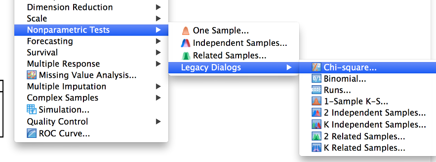
SPSS menu showing nonparametric tests, legacy dialogs, then chi-square being selected
Click on the name of the variable, and then click the arrow to move it to the “Test Variable List” box.
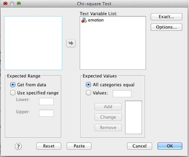
SPSS chi-square dialog
If you want to specify the proportions, you can do so using the “expected values” box. Click the radio button next to “Values,” and add each proportion to the list using the “Add” button. For example: 0.005 and 0.995. These values should add to 1.0.
Click OK.
17.3.4 Decide
Examine the output. The value of p is given as “Asymp. Sig.” (p = 0.148 in the example below so you would retain the null). The value of chi-square is given in the same table. You are also given a table with the name of your variable. It shows the proportions observed in the data along with the proportions that were predicted by the null hypothesis. The residual is the difference. As the residual grows and the proportions get further away from the predicted values, the value of chi-square increases and the value of p decreases.
If you retain the null, you conclude nothing. If you reject the null, you can conclude that the proportions are significantly different from their predicted values.
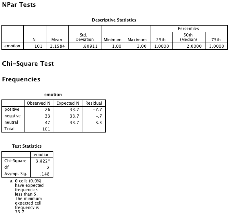
SPSS output showing Descriptive Statistics table and chi-square test
17.3.5 Conclude
The conclusion paragraph is pretty simple:
A chi-square goodness-of-fit test indicated there was a not significant difference in the proportion of individuals who rated the images as positive, negative, or neutral as compared with evenly distributed ratings, \(\chi^2\)(2, n = 101) = 3.8, p = 0.148.
- \(\chi^2\)(2 df in “Test Statistics” table (also equal to \(k\) – 1)
- , n = 101 Total Observed N
- ) = 3.8 Chi-square
- , p = 0.148 the value of Asymp. Sig.
17.4 Chi-square test for independence (two sample chi-square)
In this example, we will see if car ownership and smoking are related.
17.4.1 Data Needed
Chi-square is a test of frequencies. You need two nominal variables . Be sure to set “Values” in the “Variable View” tab of SPSS. Here, we have “car” (1 = own a car, 0 = does not own a car) and “smoke” (1 = smoker, 0 = non-smoker). Each case (row) is data from one person.
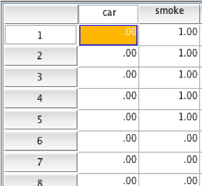
SPSS data showing car and smoke variables
17.4.2 Write Hypotheses
\(H_0\): Car ownership and smoking are independent. \(H_a\): Car ownership and smoking are not independent.
17.4.3 Check Assumptions
The minimal assumptions are random sampling from the population and independence of observations. Also, none of the expected frequencies should be zero, and most of the expected frequencies should be greater than 5.
17.4.4 Analysis
Click the “Analyze” menu, then “Descriptive Statistics,” then “Crosstabs.”
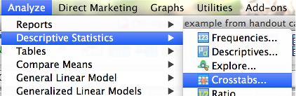
SPSS Analyze menu showing Decriptive Statistics then Crosstabs being selected
Add one variable to “Row” and the other to “Column(s).” Also check “Display clustered bar charts” (not shown in the picture).
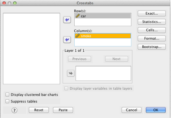
SPSS Crosstabs dialog box
Click “Statistics” and check “Chi-square” and “Phi and Cramer’s V.” Click “Continue.”
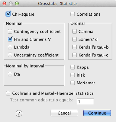
SPSS Crosstabs Statistics dialog box
Click “Cells” and check “Observed,” “Row,” “Column,” and “Total.”
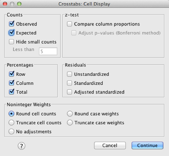
SPSS Crosstabs Cells dialog box
Click “Continue.” Click “OK.”
17.4.5 Decision
Check assumptions: Check “minimum expected count” which is listed as a footnote below the “Chi-square tests” table:
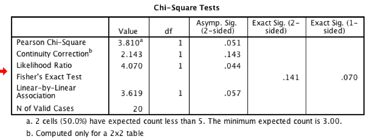
SPSS output showing Chi-Square Tests table
Earlier, we said that most of the expected frequencies should be greater than 5. Our minimum is 3 (lower than 5). From this same line, 50% of our expected frequencies are less than 5. That’s too much. We have violated the assumption of minimum expected cell frequency. Use 20% as the cutoff. If more than 20% of cells have an expected count less than 5, the assumption is violated. If this happens, either collect more data, or find an alternative technique (Fisher’s Exact Probability Test is one example).
With that out of the way, we can reject or retain the null hypothesis. Use the “Continuity correction” line, which solves some issues with chi-square tests. If this is not provided, use “Pearson Chi-Square.” Asymp. Sig (2-sided) is our p value.
17.4.6 Conclusion
Other information you need is in the “…Crosstabulation” table:
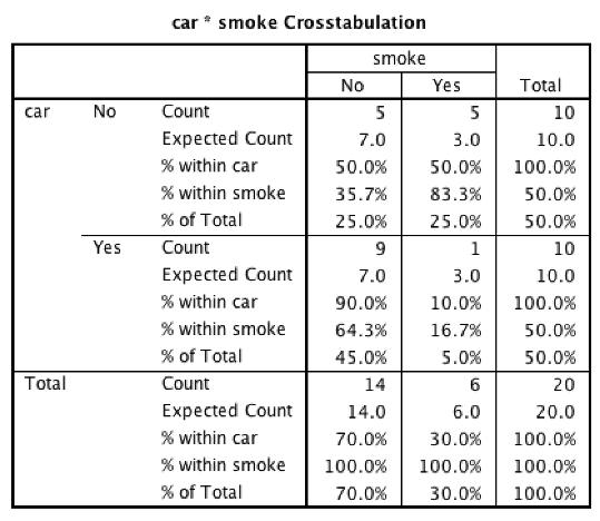
SPSS Crosstabulation table output
The two rows you need are the first ones that add up to 100%. Look for the % within [that same variable].
The table shows the observed frequencies (e.g. 9 people with a car do not smoke; 1 person with a car does smoke) and the observed relative frequencies (e.g., 90% of the people with a car are non-smokers). Use these values to interpret a significant chi-square. If this data had reached significance (it did not), we would have concluded that people who own a car are more likely to be non-smokers than smokers.
Finally, measure effect size by looking at the “Symmetric Measures” table:
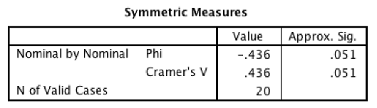
SPSS Symmetric Measures table output
17.4.7 Interpretation of \(\phi\) (phi; Cohen, 1988)
These are reference points, not firm cutoffs. For example, .29 is a medium effect size.
| Value of \(\phi\) | Effect size |
|---|---|
| \(\phi\pm.10\) | Small effect |
| \(\phi\pm.30\) | Medium effect |
| \(\phi\pm.50\) | Large effect |
17.5 Results Paragraph
A chi-square test for independence (with Yates’ correction for continuity) did not show a significant association between car ownership and smoking, \(\chi^2\)(1, n = 20) = 2.143, p = .143. A large effect was observed, \(\phi\) = -.436.
- “with Yates’…” only include this text if you see the “continuity correction” line
- \(\chi^2\)(1 df in “Chi-Square Tests” table
- , n = 20 Total count in lower-right of “…Crosstabulation” table
- ) = 2.143 Chi-square from “continuity correction” or “Pearson Chi-Square”
- , p = 0.143 the value of Asymp. Sig. (2-sided)
- A large effect see the effect size interpretation table
- \(\phi\) = -.436. Symmetric measures value