Chapter 4 The Normal Distribution & z-Scores
4.1 Normal Distributions Are Special
In statistics, normally distributed data are special. We see normal distributions in nature (sometimes). When data is normally distributed, we can make additional conclusions about it because we know its shape.
You already know three ways to determine if a distribution is normal or not (looking at the histogram, comparing the mean and median, and using SPSS). In the real world, examining the histogram along with the SPSS method is most useful.
You may have discovered in the activities that you could not create a meaningful histogram for nominal data. Here is a more formal list of the qualities of normal distributions:
- They represent continuous*, quantitative data
- They are symmetrical (so, no skew)
- The mean, median, and mode are equal
- They are bell-shaped and symmetric about the mean
- The total area under the curve is equal to 1
- The ends of the curve approach, but never touch, the x-axis (this is called an asymptote)
- As you go from the mean to past one SD away from the mean, the graph starts curving upward
* You will see this rule broken from time to time, as other kinds of distributions can sometimes be treated like continuous distributions. Likert-type scales are a good example. Technically, normality is a property of continuous data.
You also can make statements about proportions (e.g., the percent of people having a specific score) based on areas under the curve (later in this section).
4.2 Probability Density Functions (PDFs)
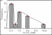
A histogram with dots at the top of each bar and a line connecting the dots
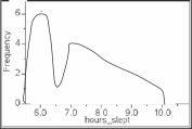
The same histogram with the bars removed, leaving only the curve
Another way to look at a histogram is as a probability density function (PDF). This means little more than connecting the midpoint of each bar to form a curve, crudely shown here:
The red dots are included to show the midpoints of each bar. Whether the graph shows bars or a continuous curve, the information is the same. When you see these curves, recognize them as showing frequencies, just like the histogram.
PDFs are a useful tool to examine the rarity of different scores. In the PDF shown above, you can see that 6.0 hours is a more common score than 10, which is more rare.
Given that PDFs are really just histograms shown as a continuous curve, we can call the normal distribution the “normal probability density function.”
4.3 Probability and Areas Under the Curve
We will discover in class that the area under the curve corresponds to probability. Three rules about probability are useful going forward:
4.3.1 Classical (or theoretical) probability: When each outcome is equally likely, the probability for an event is equal the number of outcomes in the event divided by the number of possible outcomes (all the possible outcomes are called the sample space).
Example: For the event of rolling a 1 on a die, there is one outcome in the event and 6 possible outcomes in the sample space, so the probability is 1/6, or 0.167, or 16.7%. For the event of rolling an even number on a die, there are 3 possible outcomes in the sample space, so the probability is 3/6, or 0.5, or 50%.
4.3.2 Addition rule for mutually exclusive events: When two events are mutually exclusive, add the separate probabilities to find the probability that any one of these events will occur.
Example : 5 psych majors in a class, 3 sociology majors, 2 nursing majors. What is the probability of being a psych major? Of being a nursing major? Of being either a psych major or a nursing major?
4.3.3 Multiplication rule for independent events: When one event has no effect on the probability of the other event, multiply the separate probabilities to find the probability that these two events will occur together.
Example: Probability of rolling a 6 on a die? Probability of rolling a 1? Probability of rolling a 1 followed by a 6?
Note: if one of the events is certain (already known) this rule does not apply. For example, after I flip a coin 100 times, I get 100 heads. What is the probability of getting tales on my next flip?
4.4 z-Scores
A z-Score is a single score expressed in standard deviation units. Z-scores are unit-less numbers that tell how far a score is from the mean.
Put another way: z-scores are how far a score is from the mean, expressed in standard deviation units. If you know the standard deviation and the mean, you can convert z-scores into raw scores and back again.
Common point of confusion: The shape of a frequency distribution does not change when converting to z-scores. Only the label of the x-axis changes. Why? Each raw score is associated with one z-score and each z-score is associated with one raw score. If you have two raw scores at the mean, you will have two z-scores at 0. Both histograms will have the same shape.
If you convert a variable into a z-score, you have standardized it.
Standardized means that you are setting the mean and standard deviation. In the case of the z-score, the standard deviation is set at 1 and the mean is 0. When you convert scores to z-scores, they become standardized, so that a raw score at the mean will always has a z-score of 0. However, standardizing does not change the shape of a distribution. If you started with a normal distribution of raw scores, the standardized scores will also be normally distributed. If you started out with skewed data, however, the standardized scores will remain skewed.
4.5 What do z-Scores Tell You?
z-Scores tell you how many standard deviations a score is from the mean. Z-scores of 0 are right on the mean. If I told you my test score as z = 0 in the class, you would know I scored right at the mean. If I told you my test score was z = -2, you would know that I scored 2 standard deviations below the mean. Z-scores are nothing more than standard deviation units. However, if the raw scores were normally distributed, you can make further conclusions.
4.6 Why are Normally-distributed z-Scores Useful?
When your data is normally distributed, the resulting z-scores are also normally distributed. A normal distribution of z-scores has a name: the standard normal curve. The standard normal curve has a mean of 0 (μ=0) and a standard deviation of 1 (σ=0). The z-score of normally distributed data tells you more than just the standard deviation units. Because z-scores have no units, they can be compared to other z-scores, even when the units of the variables are not the same. So you can compare relative performance across two variables that don’t have the same units.
4.7 Transforming a Raw Score into a z-Score
Transforming a raw score (X) to a z-score: \(z=\frac{X-\mu}{\sigma}\)
In words: - Find the mean of all the scores in your population (μ). - Subtract μ from the score (X). - Divide your result from step 2 by the standard deviation (σ) for the population.
4.8 Transforming a z-Score into a Raw Score
Transforming a z-score (z) to a raw score (X): \(X = \mu + (z)(\sigma)\)
In words:
- Find the mean of all the scores in your population (μ).
- Multiply the z-score by the standard deviation (σ) for the population.
- Add steps 1 and 2 to get the raw score.
4.9 Finding z-Scores in SPSS
As you cannot specify an arbitrary mean and standard deviation, you cannot always rely on SPSS for z-scores. Be sure to practice with the z-score formulas, as well.
Go to the “Analyze” menu, then select “Descriptive Statistics,” and then select “Descriptives” (not “Frequencies” this time).
Move the variable of interest over to the right.
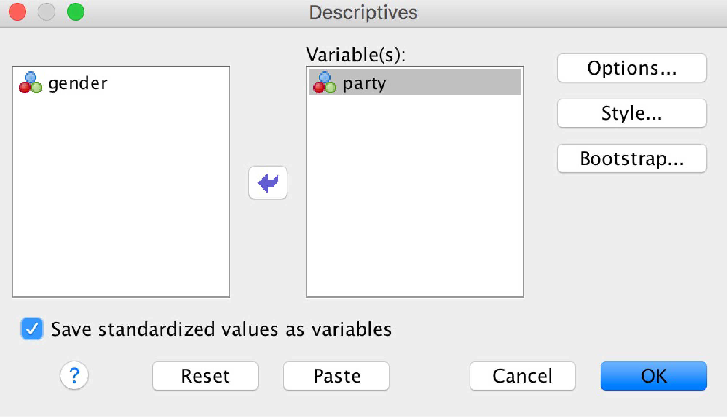
SPSS Descriptives Dialog box showing a variable moved to the right
Check the “Save standardized values as variables” checkbox. Click “OK.”
Ignore the output window. Back in your data, you’ll find one new variable has been created (in the example shown, it was called “Zparty”). SPSS has calculated the mean and standard deviation of these data and converted the scores to z-scores.
4.10 Areas Under the Curve – NormalCDF and InverseNormal
We can get even more specific; we can talk about the probability of selecting a particular score. In the graph above, if you were to select a participant at random, it is more likely that you would get someone who slept 6 hours than someone who slept 10 hours. In normally distributed data (see how the normal distribution is special in statistics), you can calculate the probability of selecting one score or a range of scores.
Finding this information is based on the area under the curve. You could calculate the area under the curve using calculus, but we need not suffer through that in this course. Instead, provided we have normally distributed data, we can look up the area under the curve in a table (or use a calculator that has this table built in, like the TI-36X Pro).
The total area under the curve is 1. To answer area under the curve problems:
Identify reference point(s) and shaded area. In the question, “find the probability of a score greater than 6,” the reference point is the raw score of 6 and the shaded area is everything above 6. In the question, “find the probability of having a score between 8 and 16,” the reference points are 8 and 16 and the shaded area is between them.
- Sketch a normal curve.
- Mark the approximate location of the reference point(s) and the mean. 3, Identify and shade the relevant area under the curve.
- Find the corresponding z-scores.
- Use your calculator to find the area of the shaded portion. The calculator shows you the area between any two reference points or a reference point and the end of the distribution. Side note: Traditionally, statistics students have been forced to use a z-table instead of a calculator. If you prefer to use a z-table, note that it shows you areas between the mean and a reference point or a reference point and the end of the distribution.
Example: The human gestation period is normally distributed with a mean of 270 days and a standard deviation of 15 days. What proportion of gestation periods will be between 245 and 255 days (Witte & Witte, 2010, p. 111)?
Sketch a normal curve. The area of interest is between 245 and 255. These are both below the mean. (If you’re curious, the corresponding z-scores are -1.67 and -1.00).
On the calculator, you can find the area between 245 (the lower bound) and 255 (the upper bound). The Normalcdf function will tell you the area between any two raw scores (or z-scores) on the normal curve. You input the lower and upper bound, population mean, and population standard deviation. The calculator will return the proportion of the curve within your bounds. See the handout specific to your calculator for instructions on using Normalcdf. Here, the answer is equal to 11.11.
Want to work in z-scores instead? Use a mean of 0 and a sigma/SD of 1 if you want to enter lower and upper bounds as z-scores instead of raw scores. In doing this, the calculator will give you the area under the curve of z-scores (a.k.a. areas under the standard normal curve).
In a variation on these problems, you will need to find the score or scores given a probability. For example, “if a baby has a gestation period in the 80th percentile, how long was the gestation period?” This problem is solved with similar steps:
- Sketch a normal curve.
- Mark the approximate location of the reference point(s) and the mean.
- Identify and shade the relevant area under the curve.
- Use the z-table or your calculator to find the z-score associated with the area.
- Find the corresponding raw scores.
The difference is which piece of information is missing. Here, we know the percentile (the proportion of area shaded under the curve), but we don’t know the score at the boundary between the shaded and unshaded regions. On the calculator, you will need to use the invNormal function to get the answer, 282.62 days.
If you’re without a calculator and stuck with a z-table, you will need to use the table backwards. Look within the table for the proportion (here, .80), find the closest labeled z-score value (z = 0.84), and convert the z-score into a raw score of 282.62.
Area-under-the-curve problems seem more difficult to master than they really are. With practice, you will identify these problems as either normalCDF or inverseNormal problems. The best way to learn this skill is to practice repeatedly.
Key points to remember:
- Every raw score from a population is associated with only one z-score, and vice-versa.
- Z-Scores are standard deviation units.
- We can make many more conclusions from normally distributed populations than we can from non-normal distributions.
- The PDF shows the same information as a histogram—frequencies.
- Because the PDF shows all the scores in the population, the area under the curve represents the probability of selecting one score at random.