Chapter 13 One-Way Analysis of Variance (ANOVA), Between-Subjects
13.1 What does ANOVA do?
ANOVA works like a t-test, but it lets you look for differences in more than 2 groups. With ANOVA, you can see if 3 groups are significantly different from each other (or 4, or 5, etc…).
ANOVA is a comparison of two kinds of variability across multiple groups.
- Between-group variability: If scores in some groups are higher or lower than other groups, then there is between-group variability. If a drug were to be effective, you would expect scores in the treatment group to be different than scores in the control group. This is the “good” kind of variability, the variability due to the treatment effect. With more between-group variability, we are more certain that the groups are different, and we are more likely to reject the null hypothesis. Between-group variability also includes variability (differences) due to random chance.
- Within-group variability: If scores within one group are different from each other, then there is within-group variability. This is the “bad” kind of variability, because we cannot provide a reason for why scores are different within one single group. In a drug trial, we wouldn’t expect participants in the treatment group to be different from one another. Differences here should be due to random chance.
ANOVA compares between-group variability to within-group variability in a ratio:
\({F}=\frac{\text{between–group variability (includes treatment effects and random chance)}}{\text{within–group variability (includes random chance)}}\)
If enough of the differences are due to the groups—between-group (and not something else we cannot explain—within-group), then we will reject the null hypothesis and conclude the groups are different.
When the null hypothesis is true, there are no treatment effects. F will be near 1. When the null hypothesis is false, more of the variability will be because of the groups. When the null is false, F will be larger than 1.
13.2 Why not Multiple T-Tests?
We could just do a series of t-tests to compare the groups. The issue is that every t-test has a 5% chance of a Type I error (or whatever the alpha level is set at). This is called the testwise error rate: The probability of a Type I error on one t-test is 5%. The probability of a Type I error on just one of several t-tests using the same data is much higher than 5%. This is called the experimentwise error rate. Ultimately, running multiple t-tests on the same data inflates the probability of a Type I error. ANOVA controls for the Type I error rate so that we can reject the null with p < .05.
13.3 Three Kinds of t-Tests, Two Kinds of ANOVA
Remember that there are three kinds of t-tests, which are used for specific research designs. Like t-tests, ANOVA has separate versions for between-subjects designs and within-subjects designs. As an introduction to the technique, we will only cover between-subjects ANOVA in this handout. Go back and review the difference between between- and within- subjects designs if needed.
13.4 One-Way Between-Subjects ANOVA – By Hand
13.4.1 Hypotheses
\(H_0:\mu_1=\mu_2=\mu3\)
in words: “the null hypothesis is that there is no difference between the means of group 1, 2, and 3.”
Note: If you have more than three groups, you need more population means.
\(H_a: H_0 \text{ is false}\)
in words: “the alternative hypothesis is that there is at least one difference between the means of group 1, 2, and 3”
13.4.2 Analysis – By Hand
In this section, we will calculate ANOVA by hand to illustrate the two sources of variability: between-group variability and within-group variability.
13.4.2.1 1. Sums and means. Calculate the following for each group:
- \(\sum{X}\) Sum (note that you will have one of these values for each group)
- \(\sum{X^2}\) Sum of each score squared
- \(M\) Mean
- \(n\) Cell size (number of participants in the group). Note that this is not overall sample size, it is only the size of one group.
Calculate the following for the entire study:
- \(\sum{X_{total}}\) Grand Sum (okay to add all the column totals)
- \(\sum{X_{total}^2}\) Grand sum of each score squared (okay to add all the column totals)
- \(M_{total}\) Grand Mean (do not use the column means; calculate this from the beginning)
- \(N\) Sample size (okay to add all the column totals)
- \(k\) The number of cells (i.e., the number of groups)
13.4.2.2 2. Sum of Squares. Calculate the total sum of squares between groups:
\(SS_{bn}=\sum{\frac{(\sum{X}^2)}{n}}-\frac{(\sum{X_{total})^2}}{N}\)
In the equation above, \(\sum{\frac{(\sum{X}^2)}{n}}\) is the sum of each: (group sum squared divided by n for the group).
The second term, \(\frac{(\sum{X_{total}})^2}{N}\) is the grand sum squared divided by sample size.
Calculate the total sum of squares:
\({SS}_{total} = \sum{X^2_{total}} - \frac{(\sum{X_{total}})^2}{N}\)
Note that \(\sum{X^2_{total}}\ne (\sum{X_{total}})^2\)
Calculate the sum of squares within groups:
\({SS}_{wn} = {SS}_{total} - {SS}_{bn}\)
13.4.2.3 3. Degrees of Freedom. Calculate the degrees of freedom between groups:
\({df}_{bn}=k-1\)
Calculate the degrees of freedom within groups:
\(df_{wn}=N-k\)
Calculate the total degrees of freedom:
\(df_{total}=N-1=df_{bn}+df_{wn}\)
- Mean Squares. Calculate the mean squares between groups:
\(MS_{bn}=\frac{SS_{bn}}{df_{bn}}\)
Calculate the mean squares within groups:
\(MS_{wn}=\frac{SS_{wn}}{df_{wn}}\)
13.4.2.4 5. F Ratio. Calculate \(F_{obt}\)
\(F_{obt}=\frac{MS_{bn}}{MS_{wn}}\)
13.4.2.5 6. ANOVA summary table. You will need this for the next steps. Write down the following numbers:
- Between: \(SS_{bn}, df_{bn}, MS_{bn}, F\)
- Within: \(SS_{wn}, df_{wn}, MS_{wn}\)
- Total: \(SS_{total}, df_{total}\)
- Decide. Use the F table to look up the critical F value (\(F_{crit}\)) using the information from your ANOVA summary table. Use α = .05 (F tests are always one-tailed). If your exact values are not in the table, use the mean of the two closest values.
- The degrees of freedom in the numerator is equal to \(df_{bn}\)
- The degrees of freedom in the denominator is equal to dfwn
- If \(F_{obt} > F_{crit}\) your F is significantly large; reject the null hypothesis
- If \(F_{obt} \leq F_{crit}\) your F is not significant; retain the null hypothesis
- Omnibus ANOVA Conclusions. With your decision, you can now make an omnibus conclusion in terms of your original groups. Did you find evidence for a significant difference between at least two of the groups?
We are missing one piece. If you reject the null, you now know that at least two groups are significantly different. But which groups are significantly different? Are all three different from each other? What if two groups had the same mean? There is a way to test the null hypothesis that two specific groups are the same. This process is called post hoc testing (testing “after the fact”). Following the omnibus ANOVA, we can test which groups are significantly different and calculate measures of effect size.
There are multiple methods of doing post hoc testing. In this course, we will use Tukey’s HSD (honestly significant difference).
13.4.2.6 9. Post-Hoc Tests
We will use Tukey’s HSD. First, look up the value of qk in the “Values of the Studentized Range Statistic” table. Note that Error df is \(df_{wn}\).
\(df_{error}=df_{wn}\)
After you find \(q_k\), compute the HSD.
\(HSD=q_k*\sqrt{\frac{MS_{wn}}{n}}\)
The HSD is the minimum difference between two means that qualifies as a “significant difference.” List each comparison (example: group 1 to group 2). For each comparison:
- Subtract the M of the first group from the M of the second group. This is the mean difference between the groups.
- If the difference is greater than the HSD, there is a significant difference between the groups.
- If the difference is less than or equal to the HSD, there is not a significant difference between the groups.
13.4.2.7 10. Effect Size
Compute an effect size for each comparison. Effect size can is measured three ways: Cohen’s d, eta squared, or by reporting the mean difference.
\(d=\frac{\bar{X}_1-\bar{X}_2}{\sqrt{MS_{wn}}}\)
Review how to interpret Cohen’s \(d\)
\(\eta^2=\frac{SS_{bn}}{SS_{total}}\)
Review how to interpret \(\eta^2\), which is the same as \(r^2\)
13.4.2.8 11. Results Paragraph
When reporting your results, you should include the results of each possible comparison. In a one-way ANOVA with 4 levels of the IV (so, four comparison groups), the groups are:
A, B, C, D
The possible comparisons you have to make are: A vs B, A vs C, A vs D, B vs C, B vs D, C vs D.
For each of these comparisons, report if the difference was significant. If it is significant, report which group is larger. Also give the mean and standard deviation of each group.
Next, we put together a complete results paragraph. In a paragraph, F is reported like this: F(df between, df within) = #.##
where df between is the df of your IV and df within is the df of the “Error” term. In this example, F would be reported as F(2, 11) = 6.30.
Use this paragraph, changing the information to reflect your data:
A one-way between-groups analysis of variance was conducted to compare groups 1, 2, and 3 on the measure. There was a significant difference between these groups, F(2, 11) = 6.30, p = .015, \(\eta^2\) = .534. Post hoc testing revealed a significant difference between scores for group 1 (M = 4.83, SD = 2.04) and group 2 (M = 9.83, SD = 2.56) and between group 1 and group 3 (M = 11, SD = 5.66). No significant difference was found between group 2 and group 3.
Exploded version of this paragraph:
- A one-way between-groups analysis of variance was conducted Name of the analysis
- to compare groups 1, 2, and 3 **Instead of “groups 1, 2, and 3” list the levels of your IV
- on the measure. List the name of the DV**
- There was a significant difference between these groups, Did you reject or retain the null?
- F(2, Degrees of freedom between
- Degrees of freedom within
- = 6.30, Value of F
- p = .015, Value of p (use p = if you have an exact value. Use p < .05 if you are using a table)
- \(\eta^2\) = .534. Partial eta squared
- Post hoc testing revealed a significant difference between scores for group 1 (M = 4.83, SD = 2.04) and group 2 (M = 9.83, SD = 2.56) and between group 1 and group 3 (M = 11, SD = 5.66). No significant difference was found between group 2 and group 3. List all possible pairs and their significance. List means and standard deviations for each group the first time you mention them.
13.5 One-Way Between-Subjects ANOVA – SPSS
13.5.1 Hypothesize
\(H_0:\mu_1=\mu_2=\mu_3\)
in words: “the null hypothesis is that there is no difference between the means of group 1, 2, and 3.” Add additional means if you have more groups.
\(H_a: H_0\text{ is false}\)
in words: “the alternative hypothesis is that there is at least one difference between the means of group 1, 2, and 3.” Add additional means if you have more groups.
13.5.2 Analyze
Select “Analyze” then “General Linear Model” then “Univariate.”
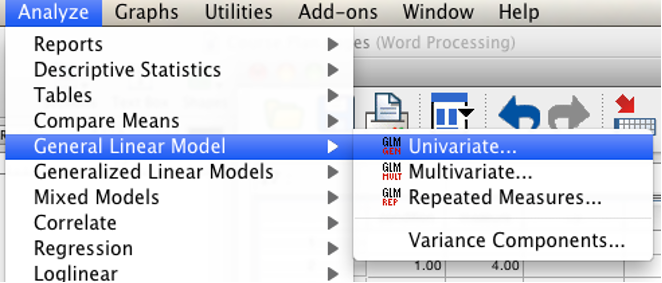
SPSS Analyze menu showing General Linear Model and then Univariate selected
Move the dependent variable into the “Dependent Variable” box. Move the grouping variable (the IV) into the “Fixed Factor(s)” box.
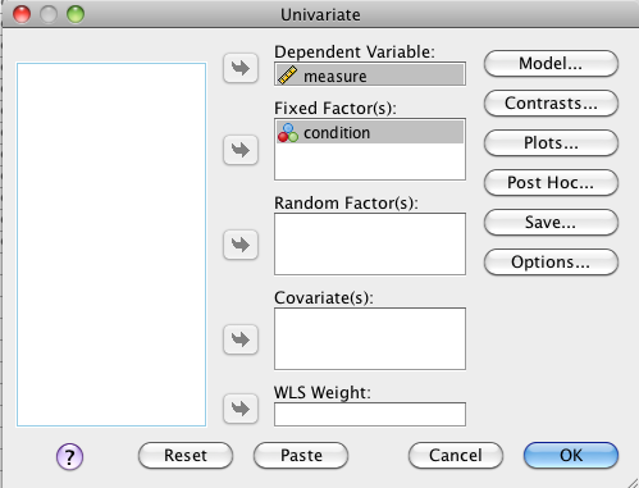
SPSS Univariate dialog box
Click “Options.” Check “Descriptive statistics,” “estimates of effect size,” and “homogeneity tests.” Click “Continue.”
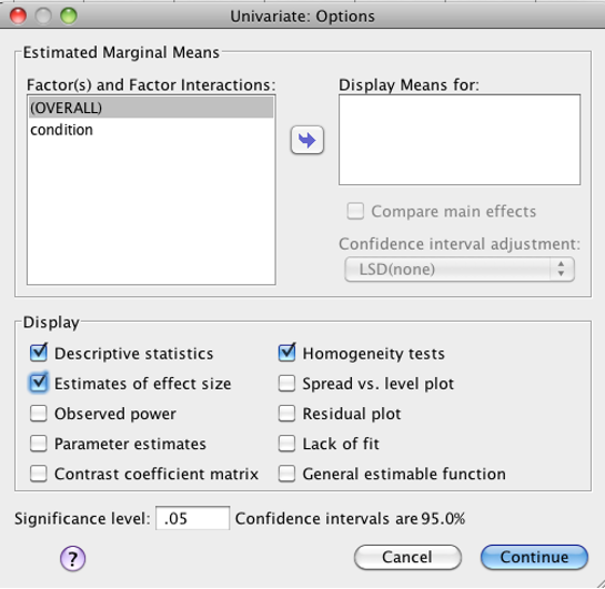
SPSS Univariate Options dialog box
Click “Post Hoc…” and move your independent variable from the “Factor(s)” list to the “Post Hoc Tests for” list. Check “Tukey” and then click “Continue.”
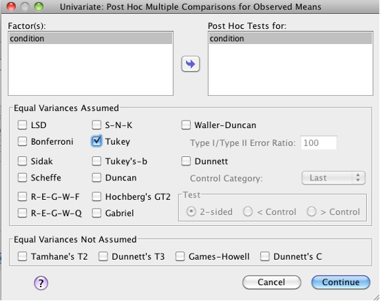
SPSS Univariate post hoc multiple comparisons dialog box
Click “OK.”
13.5.3 Check Assumptions
Homogeneity of Variances: You check this after your test is run. Examine the output for Levene’s Test for Homogeneity of Variances. If “Sig.” value is larger than .05, you have not violated the assumption. If Sig. value is less than .05, you have violated the assumption. If violated, you can’t really trust the results. Solutions to this problem are outside the scope of this course. One option is to re-run the ANOVA using the “One Way ANOVA” in the “Compare Means” section of the “Analyze” menu and checking “Welsh” and “Brown-Forsythe” in the options screen.
13.5.4 Decide
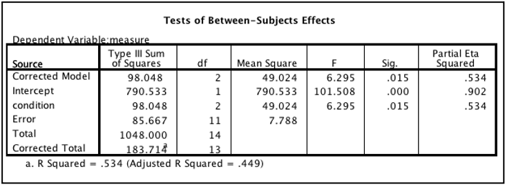
Look for your IV in the “Tests of Between-Subjects Effects” table. Then find the “Sig.” column. This value is the p value of your test.
If p is less than .05, then you reject the null hypothesis (there is a significant difference between the groups).
If p is greater than or equal to .05, then you retain the null hypothesis (no conclusions can be made)
 ### Conclude
If you retained the null hypothesis, you can stop here. There is nothing to conclude.
### Conclude
If you retained the null hypothesis, you can stop here. There is nothing to conclude.
If you rejected the null, you must take a look at the post hoc tests to see which pairings are significant. For example, there may be a significant difference between the means of group 1 and group 2, but not between group 2 and group 3.
13.5.5 Post Hoc Tests
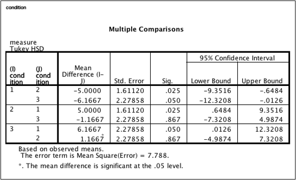
Look for the “Multiple Comparisons” table. This table lists comparisons between every combination of two levels of your IV. In the example below, the first line is the comparison between condition 1 and condition 2. Notice that each pairing is repeated (condition 1 vs condition 2 is the same comparison as condition 2 vs. condition 1).
Check the “Sig.” value of each comparison. Remember than in SPSS, “Sig” is p. For each comparison, if p is less than .05, then you reject the null hypothesis (there is a significant difference between the groups). If p is greater than or equal to .05, then you retain the null hypothesis (no conclusions can be made about that pair).
SPSS Multiple Comparisons table
In this example, there is a significant difference between condition 1 and condition 2. There is not a significant difference between condition 1 and condition 3 (note the somewhat unusual situation of p being exactly, not less than, .05). There is not a significant difference between condition 2 and condition 3 (p is much greater than .05). What does this mean? To make sense of the post hoc tests, you always have to go back to the group means:
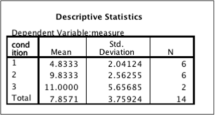
SPSS Descriptive Statistics table
Participants in condition 1 had significantly lower scores than those in condition 2. Participants in condition 1 also had significantly lower scores than those in condition 3. However, the 1.67 unit difference between condition 2 and 3 was not significant.
13.5.6 Effect size
Partial eta squared is provided in the “Test of Between-Subjects Effects” table. Remember to use the row that has the name of your IV.
Review how to interpret \(\eta^2\), which is the same as \(r^2\)
Note: Partial eta squared is not the same thing as eta squared. In a one-way ANOVA like this one, however, partial eta squared equals eta squared. In a factorial ANOVA (covered later), partial eta squared is variance accounted for by one factor without variance accounted for by other factors. You can avoid this mess by always reporting one-way ANOVA results as “eta squared” (or, better yet, \(\eta^2\)).
13.6 Results Paragraph
You will need the value of F (in the example it’s 6.295). F is reported like this:
F(df between, df within) = #.##
where df between is the df of your IV and df within is the df of the “Error” term. In this example, F would be reported as F(2, 11) = 6.30.
Next, we put together a complete results paragraph. Use this paragraph, changing the information to reflect your data:
“A one-way between-groups analysis of variance was conducted to compare groups 1, 2, and 3 on the measure. There was a significant difference between these groups, F(2, 11) = 6.30, p = .015, \(\eta^2\) = .534. Post hoc testing revealed a significant difference between scores for group 1 (M = 4.83, SD = 2.04) and group 2 (M = 9.83, SD = 2.56) and between group 1 and group 3 (M = 11, SD = 5.66). No significant difference was found between group 2 and group 3.
Exploded version of this paragraph:
- A one-way between-groups analysis of variance was conducted Name of the analysis
- to compare groups 1, 2, and 3. Instead of “groups 1, 2, and 3,” list the levels of your IV
- on the measure. List the name of the DV
- There was a significant difference between these groups, Did you reject or retain the null?
- F(2, Degrees of freedom between
- Degrees of freedom within (“df Error”)
- = 6.30, Value of F
- p = .015, Value of p (use p = if you have an exact value. Use p < .05 only if you are using a table)
- \(\eta^2\) = .534. Eta squared (labeled partial eta squared in SPSS)
13.6.1 Confidence intervals and point estimates
Confidence intervals (“95% confidence interval”) and parameter estimates (“Mean Difference”) are provided as part of the post hoc test. Look for the “Multiple Comparisons” table.
SPSS Multiple Comparisons