Chapter 14 One-Way Analysis of Variance (ANOVA), Within-Subjects

14.1 Within-Subjects ANOVA vs Between-Subjects ANOVA

The design of the study determines which ANOVA is used. Within-subjects ANOVA (for within-subjects designs) is also called repeated measures ANOVA.

Here is an example data file:

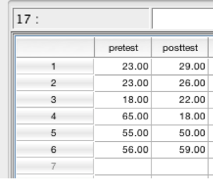
SPSS data showing pretest and posttest

Note the differences in the data file for a within-subjects design. There is no grouping variable. All participants received the same treatment so there are no groups. The only “group” is time (measurement at time 1, pretest, versus measurement at time 2, posttest). While each participant is still represented by one row, each column represents a measurement at one point in time.

With only a pretest and posttest score, we could have analyzed this data using either a paired samples t-test or within-subjects ANOVA. Unlike the t-test, the ANOVA allows us to have more than 2 groups.

14.2 The F Ratio

The F ratio in within-subjects design is similar to the F statistic in a between-subjects design. A key difference is that there is no longer an assumption of independence between treatment groups. Instead, the scores are assumed to be related. For example, the participant measured at time 1 is the same participant measured at time 2. Because of that assumption, individual differences are removed before the calculation of F.

\(F=\frac{\text{between–group variability (includes treatment effects and random chance), but no individual differences due to design}}{\text{within–group variability (includes random chance), with variability due to individual differences removed}}\)

14.3 One-Way Repeated Measures ANOVA (Within-Subjects) - SPSS

14.3.1 Hypotheses

Hypotheses are written the same as for between-subjects ANOVA. The difference here is that the same people are in “group” 1 and in “group” 2.

\(H_0: \mu_1=\mu2\) (include one population mean for each level of the IV) \(H_a:H_0 \text{ is false}\)

14.3.2 Analysis

“Analyze” then “General Linear Model” then “Repeated Measures.”

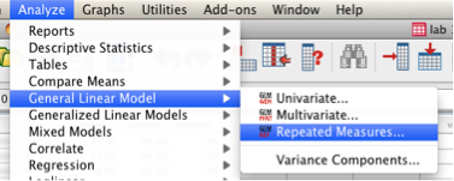
SPSS Analyze menu showing General Linear Model and Repeated Measures selected

The “Define Factor(s)” box will appear. You now have to enter the names of your IV and DV. Here, our IV can be described as time, so enter time as the “Within-Subject Factor Name” and enter 2 levels (because our IV has two levels, time 1 and time 2). Then click Add.

In the “Measure Name” box, put the name of your dependent variable (DV). Then click Add. Then click “Define.”

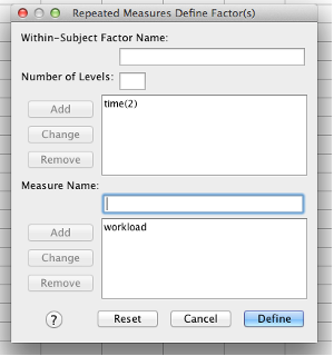
SPSS Repeated Measures Define Factor(s) dialog box

Now, you can select your variables. Move each variable representing the DV over to the “Within-subjects variables” box. The number of variables that you include is based on what you typed into the previous “Define Factor(s)” box: You will have one line in the “Within-Subjects Variables” box for each level of your within-subjects IV. This process is very similar to a paired-samples t-test.

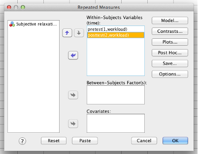
SPSS Repeated Measures dialog box

Click “Options.” You want to move everything over to the “Display Means for” box. Also check the “Compare main effects” checkbox. Check “Descriptive statistics” and “estimates of effect size.”

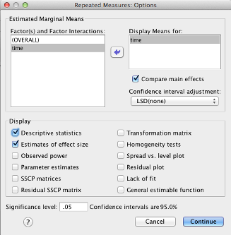Click “Continue,” then click “OK.”

14.3.3 Check Assumptions

Sphericity: As long as you use the “Multivariate tests” table instead of “tests of within-subjects effects,” you do not have to worry about violating the assumption of sphericity. Sphericity is an important assumption in repeated measures ANOVA. Violating it unknowingly can lead to an inflated Type I error rate.

If you’re curious: The differences between each score for each participant (for example, time1 - time2) form a distribution. For each pairing of your conditions (time1 - time3, time2 - time3, etc.), you can create one of these distributions. Sphericity is when the variance of each of these distributions is equal. If the Sig. value for Mauchly’s test is significant, you have violated the assumption of sphericity. If there is only “.” shown, then you do not have enough groups (3 or more) for sphericity to be an issue.

14.3.4 Decide

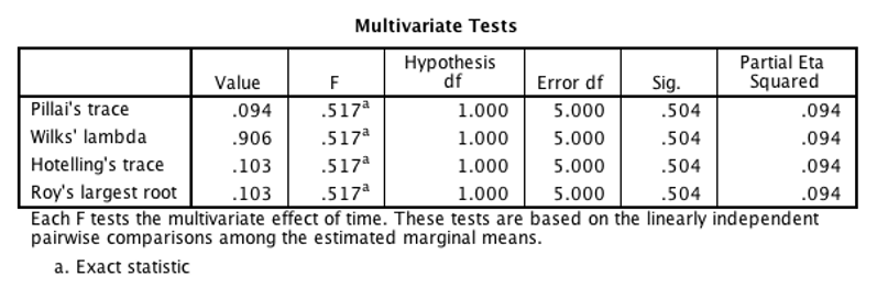
Look for the “Multivariate Tests” table. Wilks’ Lambda is the most commonly reported statistic; use that one. The Sig. value is the p value for this test. If p is less than .05, then you reject the null hypothesis (there is a significant difference between the levels) . If p is greater than or equal to .05, then you retain the null hypothesis (no conclusions can be made). In the example shown, we retain the null hypothesis because Sig. is greater than 0.05.

SPSS output Multivariate Tests table

14.3.5 Post Hoc Tests

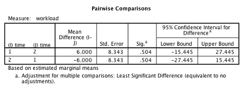
The post hoc tests are in the “Pairwise comparisons” table. This example was not significant. If this were a real-world example, we would not do post hoc tests for that reason. Additionally, there are only two levels for the IV in the example shown. If the omnibus ANOVA is significant when there are only two levels of the IV, you know that the single comparison is significant.

In cases where you have 3 or more levels of your between-subjects IV and a significant result, you would do a post hoc test on each comparison. In the example below, our single post hoc test is between time 1 and time 2. It is not significant (p = .504).

SPSS output Pairwise Comparisons table

14.3.6 Conclude

You will need the value of F (in the example it’s 0.517). F is reported like this: F(df between, df within) = #.##. Degrees of freedom between is called “hypothesis df” in the “Multivariate Tests” table and df within is called “error df” in the same table. In this example, F would be reported as F(1, 5) = 0.52.

Report your results the same way as the between-subjects ANOVA. Include all the same statistics: “A within-groups analysis of variance was conducted to compare workload before and after the math test. There was no significant difference between the two measurements, F(1, 5) = 0.52, p = .504, partial \(\eta^2\) = .094.”

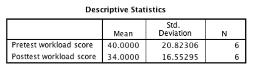
But what if the Sig. value had been less than .05? If the omnibus test was significant, you would continue to post-hoc testing. When reporting post-hoc results, you must report the means and SDs of each level of the IV. Find the “Descriptive Statistics” table. Each post-hoc comparison will add another sentence to the paragraph:

“Post hoc testing did not reveal a significant difference between workload before the math test (M = 40.00, SD = 20.82) than after (M = 34.00, SD = 16.55).”

This example included only 2 levels, so there would only be one comparison. Keep in mind that when the omnibus ANOVA is significant, you need to report post-hoc results for each possible comparison.

Finally, it’s important to interpret the meaning of your results. Always look back at the means of each group to interpret the meaning. In the example below, we conclude that workload was higher after the posttest. Therefore, our manipulation increased workload.

SPSS output Descriptive Statistics table