Chapter 15 Two-Way Analysis of Variance (ANOVA)

15.1 Interactions

Interactions are also called moderated relationships or moderation. An interaction occurs when the effect of one variable depends on the value of another variable.

For example, how do you increase the sweetness of coffee? Imagine that sweetness is the DV, and the two variables are stirring (yes vs no) and adding a sugar cube (yes vs no). We can draw the impact of these two factors (factor is a fancy word for IV) in a table:

.	Stirring: Yes	Stirring: No
Sugar: Yes	\(\bar{X}_{sweet}=100\)	\(\bar{X}_{sweet} = 0\)
Sugar: No	\(\bar{X}_{sweet}=0\)	\(\bar{X}_{sweet} = 0\)

When is the coffee sweet? Stirring alone does not change the taste of the coffee. Adding a sugar cube alone also doesn’t change the taste of the coffee since the sugar will just sink to the bottom. It’s only when sugar is added and the coffee is stirred that it tastes sweet.

We can say there is a two-way interaction between adding sugar and stirring coffee. The effect of the stirring depends on the value of another variable (whether or not sugar is added).

Drawing an ANOVA means table is a good way to understand interaction effects. To draw this table, place one factor on each axis, as shown above. Then, include every possible mean in the boxes.

15.2 Some Terminology

When more than one IV is included in a model, we are using a factorial design. Factorial designs include 2 or more factors (or IVs) with 2 or more levels each. In the coffee example, our design has two factors (stirring and adding sugar), each with two levels. An ANOVA with two-factors is called a two-way ANOVA. Previously, we looked at one-way ANOVAs, those with only one factor.

In factorial designs (i.e., studies that manipulate two or more factors), participants are observed at each level of each factor. Because every possible combination of each IV is included, the effects of each factor alone can be observed. We also get to see how these factors impact each other. We say this design is fully crossed.

15.3 Main Effects

A main effect is the effect of one factor. There is one potential main effect for each factor.

In this example, the potential main effects are stirring and adding sugar. To find the main effects, find the mean of each column. If there are differences in these means, there is a significant main effect for one of the factors. Next, find the mean of each row. If there are differences in these row means, then there is a main effect for the other factor.

.	Stirring: Yes	Stirring: No	Row mean
Sugar: Yes	\(\bar{X}_{sweet}=100\)	\(\bar{X}_{sweet} = 0\)	\(\bar{X}_{sugar}= 50\)
Sugar: No	\(\bar{X}_{sweet}=0\)	\(\bar{X}_{sweet} = 0\)	\(\bar{X}_{\text{no sugar}}=0\)
Column mean	\(\bar{X}_{stir}=50\)	\(\bar{X}_{nostir}=0\) .

In our example, we see two main effects. Adding a sugar cube (mean of 50) differs from not adding sugar (mean of 0). That’s the first main effect. The second is stirring; stirring (mean of 50) differs from not stirring (mean of 0).

15.4 Simple Effects

When an interaction effect is present, each part of an interaction is called a simple effect. To examine the simple effects, compare each cell to every other cell in the same row. Next, compare each cell to ever other cell in the same column. Simple effects are never diagonal from each other.

In our example, we see a simple effect as we go from Stir+Sugar to NoStir+Sugar. There is no simple effect between Stir+NoSugar and NoStir+NoSugar (both are 0). What makes this an interaction effect is that these two simple effects are different from one another.

On the vertical, there is a simple effect from Stir+Sugar to Stir+NoSugar. There is no simple effect from NoStir+Sugar to NoStir+NoSugar (both are 0). Again, this is an interaction effect because these two simple effects are different.

15.5 Interaction Effect

When there is at least one (significant) simple effect that differs across levels of one of the IVs (as demonstrated above), then you can say there is an interaction between the two factors. In a two-way ANOVA, there is one possible interaction effect. We sometimes show this with a multiplication symbol: Sugar*Stir. In our example, there is an interaction between sugar and stirring.

15.6 Factorial ANOVA is really 3 ANOVAs

When evaluating main effects, simple effects, and interactions, how do you know how much of a difference is enough? Great question! This is why we do significance testing. Running the two-way ANOVA lets you see whether you have main effects and/or an interaction effect.

When you run a two-way ANOVA, you are really running three ANOVAs:

• An F-test of the interaction.
• An F-test of the first factor.
• An F-test of the second factor.

Any combination of these can reach significance (or not).

15.7 Interpret Interaction Effects First

When you interpret a two-way ANOVA, you need to always start with the interaction. Sometimes, significant main effects with a significant interaction are misleading. Significant main effects might be fully explained by the interaction.

In our example, you may have noticed a discrepancy. We started by saying that adding sugar or stirring alone did not affect the sweetness of the coffee. But, when we analyzed the table, we saw two main effects. This illustrates why we always need to look at our interaction effects first, and then take a closer look at the means, before we interpret main effects.

Merely reporting the SPSS output would lead us to conclude that stirring has an effect, adding sugar has an effect, and the interaction has an effect. This is not the case. While, on average, stirring lead to sweeter coffee, it was only sweeter when sugar was also added. Always interpret significant interaction effects first.

15.8 Hypotheses

You need a set of hypotheses for each factor and one for the interaction. Note that the number of means depends on the number of levels for each factor.

For “factor A”:

$H_0:\mu_{A1}=\mu_{A2}=\mu_{A3}$ 
$H_a:H_0\text{ is false}$

For “factor B”:

$H_0:\mu_{B1}=\mu_{B2}$ 
$H_a:H_0\text{ is false}$

For the interaction:

$H_0:\text{there is no interaction between test difficulty and training}$
$H_a:H_0\text{ is false}$

15.9 Analysis Two-Way ANOVA (Between-Subjects, Within-Subjects, or Mixed Model)

15.9.1 Differences from One-Way ANOVA

Running a two-way ANOVA is essentially the same procedure as a one-way ANOVA except that you will add a second factor (IV). The following sections focus on the differences between two-way and one-way ANOVAs in SPSS. You will need to refer back to the relevant one-way ANOVA sections.

15.9.2 Analyzing fully Between-Subjects Designs

If you have two (or more) between-subjects factors, run a regular between-subjects ANOVA, but include multiple factors in the “Fixed Factor(s)” box.

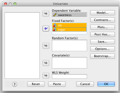
SPSS Univariate Box

In the “Options” screen, make sure you include both IVs in the “Display means for” box.

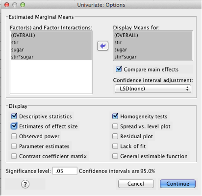
SPSS Univariate Options dialog box

Click “Post Hoc” and make sure you include both IVs in the “Post Hoc Tests for” box.

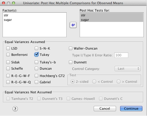
SPSS Univariate Post Hoc dialog box

Finally, click “Plots” and add one factor to the “Horizontal Axis” box and the other to the “Separate Lines” box. Then click “Add.” FYI, if you had a three-way ANOVA, you could include a third factor in the “Separate Plots” box. Click “Continue.” This will generate graphs of the means at the end of your output, which will be helpful later.

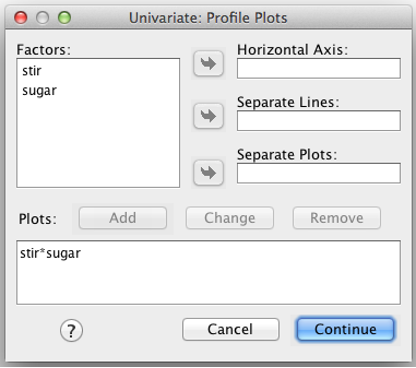
SPSS Plots

Before you click “OK,” to run your analysis read the following section titled “SPSS Drops the Ball on Simple Effects Tests.”

15.9.3 Analyzing fully Within-Subjects Designs

If you have two (or more) within-subjects factors, run a regular within-subjects ANOVA. However, “Add” more than one “Within-Subject Factor Name” to the first box:

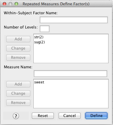
SPSS Repeated Measures Define Factor(s) dialog box

Note what you get when you click “Define”:

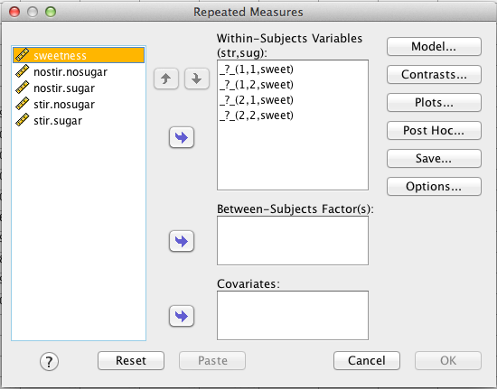
SPSS Repeated Measures dialog box

Here, SPSS asks you for every single cell, in order. In a within-subjects factorial design, you need one SPSS variable for every cell.

The first variable is (1,1,sweet). See the text just above the box: “(str, sug).” The first variable is str = 1, sug = 1 (nostirring and nosugar). The next variable is str = 1, sug = 2 (nostirring and sugar), and so on.

Next, click “Options.” Be sure everything is moved over to the “Display Means for” box and that “Compare main effects” is checked. Also check “Descriptive statistics,” “estimates of effect size,” and “homogeneity tests.” Click “Continue.”

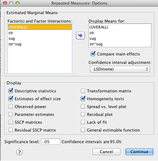
SPSS Repeated Measures Options dialog box

A quick note about the homogeneity tests: They only apply to mixed designs (below). You will see an error message with fully within-subjects designs; this is normal.

Next, click “Post Hoc” and make sure you include both IVs in the “Post Hoc Tests for” box. Check “Tukey.”

Finally, click “Plots” and move one factor to “horizontal axis” and the other factor to “separate lines.” Click “Add,” then click “Continue.”

Before you click “OK,” to run your analysis, read the following section titled “SPSS Drops the Ball on Simple Effects Tests.”

15.9.4 Analyzing Mixed Designs

It is also possible to have one between-subjects factor and one within-subjects factor. This is called a mixed design. To run a mixed design, follow the procedure above for within-subjects design. The only change is to include a grouping variable in the “Between-Subjects Factor(s)” box. The grouping variable adds a between-subjects IV to your model.

Important: To run a mixed design, start with the procedure for within-subjects designs. You can include a between-subjects factor in the SPSS Repeated Measures procedure, but you cannot do the opposite (i.e., there is no option to add a within-subjects factor in the SPSS Univariate procedure).

Before you click “OK,” to run your analysis, read the following section titled “SPSS Drops the Ball on Simple Effects Tests.”

15.9.5 SPSS Drops the Ball On Simple Effects Tests

You should be aware of a limitation in SPSS that nobody seems to talk about. You will not get Sig. values for the simple effects in an interaction. You will get means but not significance values. There are two ways to handle this:

Option 1: Just look at the means and the graph in your output. Give an interpretation of the results without saying which differences are significant. This will probably be fine unless you want to publish in a journal. In this course, you should use the second method:

Option 2: Force SPSS to give you the Sig. value you want. Apply either no correction or apply a Bonferroni correction to control Type I error. “No correction” is a bit liberal, which increases your chance of a Type I error as you make more comparisons. However, Bonferroni is too conservative (you might end up committing a Type II error). In this section, we will use “no correction.”

Here is how to get the simple effects tests you need:

Before you run a factorial ANOVA, don’t click “OK.” Click “Paste.” Clicking “Paste” takes your entire analysis and turns it into code that you can run later. This is a handy feature for real-world data, because you can run the same analysis again in the future.

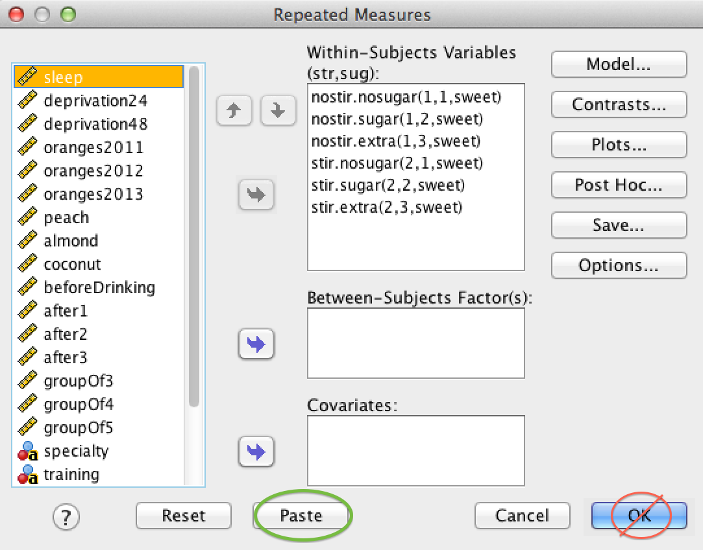
SPSS Repeated Measures dialog box showing location of Paste button

A new window opens with SPSS Syntax. Remain calm; we are going to make one small change:

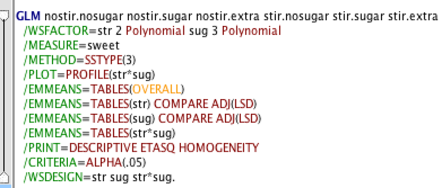
SPSS syntax window showing result of clicking the paste button

Find the /EMMEANS line for the interaction. Look for *. In this example, it’s the 9th line.

After that line, tap the space bar. Then add:

COMPARE(str) ADJ(LSD)

“Str” is just for this example. Instead of “str,” you need to use the name of the first factor in the interaction. If you want to do the more conservative Bonferroni correction instead, type BONFERRONI instead of LSD. With that addition, the line should now read:

/EMMEANS=TABLES(str*sug) COMPARE(str) ADJ(LSD)

Highlight everything, and click play: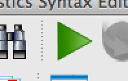. You can also select “Run All” from the “Run” menu.

Your analysis will run, and you will get an output. Your interaction table will become a “Pairwise comparisons” table. When you write your paragraph, you do not need to report the p values, but you should report which differences were significant.

If you would like to read more about this problem, see this document from the software developer: http://www-01.ibm.com/support/docview.wss?uid=swg21475404

15.10 Check Assumptions

You need to check the same assumptions for each factor (and the interaction) that you would for a one-way ANOVA:

If one or both factors are between-subjects, you need to check Homogeneity of Variances: Examine the output for Levene’s Test for Homogeneity of Variances. If “Sig.” value is larger than .05, you have not violated the assumption. If Sig. value is less than .05, you have violated the assumption. If violated, you can’t really trust the results. Solutions to this problem are outside the scope of this course. One option is to re-run the ANOVA using the “One Way ANOVA” in the “Compare Means” section of the “Analyze” menu and checking “Welsh” and “Brown-Forsythe” in the options screen.

If one or both factors are within-subjects, sphericity is not an issue so long as you stick with the “Multivariate tests” table (described below).

15.11 Decision

Remember, you have three omnibus decisions to make: Factor 1, Factor 2, and the interaction.

Start with the omnibus tests. You have to decide if you are going to reject the null hypothesis for factor 1. Then, you have to decide if you are going to reject the null hypothesis for factor 2. Finally, you have to decide if you are going to reject the null hypothesis for the interaction.

The table where you find this information depends on what kind of factor you have (between or within)

15.11.1 Omnibus Tests for Between-Subjects Design or the Between-Subjects Factor in a Mixed Design

If you have a between-subjects factor, SPSS will give you a “Tests of Between-Subjects Effects” table. Interpretation of this table is the same as it was for one-way between-subjects ANOVA.

If you have a fully between-subjects design, the omnibus test for the interaction effect will also appear in this table.

SPSS output showing Tests of Between-Subjects Effects table

Here, both of the main effects, stir and sugar, are significant (p < .001) with outrageous F values (it’s fake data).

The interaction, stir * sugar, is also significant.

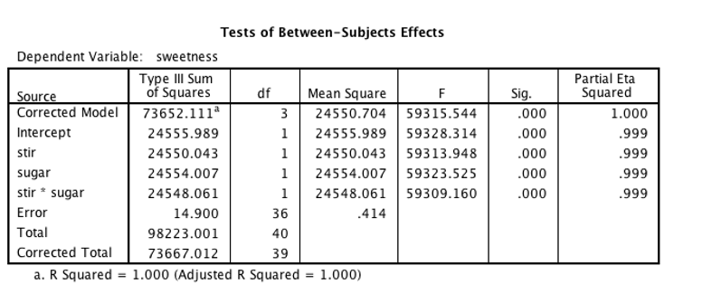
15.11.2 Omnibus Tests for Within-Subjects Design or the Within-Subjects Factor in a Mixed Design

As with one-way ANOVA, the Multivariate Tests table has what you need without the assumption of sphericity. You will see one test for each within-subjects factor.

If you have a fully between-subjects design or a mixed design, then the omnibus test for the interaction effect will also appear in this table.

SPSS output showing Multivariate Tests table

15.11.3 Post Hoc Tests

For each significant factor with 3+ levels or a significant interaction, you need to do post hoc testing. If you have only two levels of a factor, you can skip post hoc testing for that factor. Consequently, you may have as many as three separate post hoc tests for one two-way ANOVA.

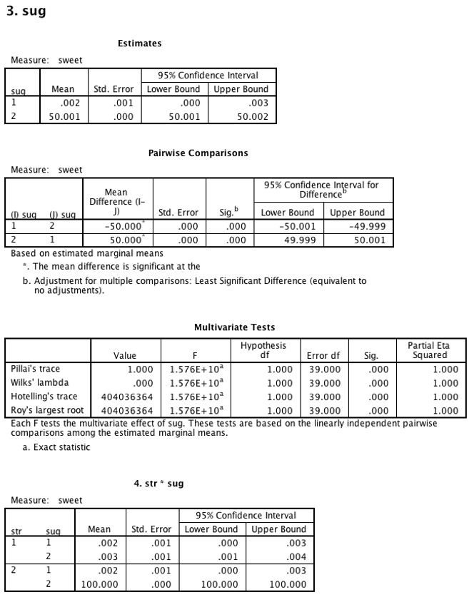
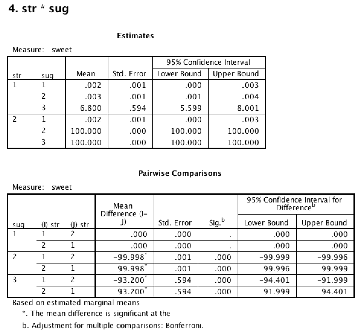
SPSS will add one section to the bottom of the output for each one of your factors. In this example, the sugar factor post-hoc tests are under a heading labeled “3. sug.”

Interpretation is the same as in one-way ANOVA. The table you need is called “Pairwise comparisons” instead of “Multiple comparisons,” but the information is the same. This example shows a repeated-measures design.

Because you used the syntax procedure listed in this section, you will also get a table for the interaction. This table shows all simple effects along with a significance value. The table for the interaction lists the mean and standard error of each cell along with a significance value. If you are missing this table, and you had a significant interaction effect, then see the section “SPSS Drops the Ball on Simple Effects Tests.”

Recall our discussion of simple effects. To interpret the interaction, first generate a list of all the significant simple effects, including their directions (i.e., which mean is larger, which mean is smaller). Your significant interaction means that this pattern is not consistent across all levels of one factor. The challenge is to tell a story based on your pattern of simple effects. In the example shown, the story of the interaction is that stirring causes coffee to be sweet, but only when sugar is added (levels 2 and 3 of sug).

15.12 Conclusion

The conclusion builds on what you have learned. Start by reporting the interaction omnibus test. Then, describe the pattern of significant simple effects with means and SEs. Finally, report any main effects, keeping in mind that they might be explained by the interaction.

“A 2x2 between-subjects ANOVA was conducted to assess the impact of stirring and adding sugar to coffee. There was a significant interaction between stirring and adding sugar, F(1, 36) = 59,309.16, p < .001, partial eta squared = .999. Driving the interaction was a significant difference in sweetness when sugar was added and the coffee was stirred (M = 100, SE = 0). This mean was significantly higher than both sugar with no stirring (M = .002, SE = .001) and no sugar with stirring (M = .003, SE = .001).

There was a significant main effect for stirring, F(1, 36) = 59,313.95, p < .001, partial eta squared = 1.00. On average, stirring lead to sweeter coffee (M = 66.67, SE = 0) than not stirring (M = 2.27, SE = 0.20). However, this main effect was explained by the interaction.

There was a significant main effect for sugar, F(1, 36) = 59,323.53, p < .001, partial eta squared = 1.00. On average, adding sugar led to sweeter coffee (M = 50.00, SE = 0) than not adding sugar (M = 0.002, SE = 0.001). However, this main effect was explained by the interaction.”

15.13 Graphing Interactions

An interaction graph is simply a plot of the means for each cell in the ANOVA. Interaction graphs make it easier to interpret your data. Remember that you need post hoc tests in order to know which differences are significant.

See: Rovira, E., McGarry, K., & Parasuraman, R. (2007). Effects of imperfect automation on decision making in a simulated command and control task. Proceedings of the Human Factors and Ergonomics Society Annual Meeting, 49(1), 76-87. Santa Monica, CA: Human Factors and Ergonomics Society. doi:10.1518/001872007779598082

The image in Rovira et al. (2007) shows a 2 x 8 repeated measures ANOVA. The two within-subjects IVs are automation failure number (8 levels) and automation type (2 levels, high and medium). The DV is correct response rate.

Steps in graphing an interaction:

1. Place the DV along the Y-axis.
2. Place factor 1 along the x-axis. It’s best to use the factor with the most levels here.
3. Use separate lines for each level of factor 2. Distinguish the lines by making one a dashed line, or use different end points for each line.
4. Plot the mean of each cell.

Steps in interpreting an interaction graph:

• If the lines are not parallel then there is an interaction effect.
• Draw a line bisecting the two lines (it cuts the angle formed by them in half). If this new line has a positive or negative slope (that is, it’s not a horizontal line), then there is a main effect for factor 1.
• If both lines have positive slope (they go up) or both lines have a negative slope (they go down) then there is a main effect for factor 1.
• If the two lines do not meet on the graph then there is a main effect for factor 2.

Remember, you do not know if these differences are significant without doing NHST.

This applet - Java required lets you manipulate means to see how the interaction graph changes: