Chapter 10 T-Tests
10.1 Experimental Design: Between-Subjects vs Within-Subjects
Experiments and quasi-experiments have a manipulation: the researcher assigns participants to different levels of the independent variable. To assess the effects of a drug, a researcher might compare a group getting the drug to a group not getting the drug (a placebo or sugar pill). The manipulation, the drug, has two levels: drug and no drug.
There are two ways to design a manipulation. Either the experimenter chooses who is in what group (between-subjects) or at what point in time each subject is in each condition (within-subjects). Between-subjects design is manipulating across different people (participants are only exposed to one level of the IV during the research). Within-subjects designs are also called repeated measures. Within-subjects designs have every participant exposed to every level of the IV. Some manipulation is done in between repeated measures. So, a drug might be given and the participant measured. Then, the drug is taken away and the participant is measured again.
An example of between-subjects design: I give one half of randomly selected participants caffeinated soda and I give the other participants caffeine free soda.
An example of within-subjects design: Participants complete anxiety surveys every day for a month. On half of the days, at random, all participants are given a placebo. On the other half of the days, all participants are given the experimental anxiety drug. In within-subjects design, participants serve as their own controls (the comparison is across trials).
10.2 Differences between groups
T-tests are a kind of analysis technique that tests for differences between groups.
In general, these techniques can be used when the independent variable(s) is/are discrete. These techniques differ in the number of IVs allowed and whether between-subjects or within-subjects designs are used.
10.3 Degrees of Freedom
In t-tests, critical values (and p-values) are based on degrees of freedom. Degrees of freedom (df), are the number of values free to vary given some constraint. Put another way, degrees of freedom are the number of values that provide information about variability. If you know only your score on the last exam, you have no way of estimating variability of test scores in class (df = 0). If you know your score and another classmate’s, you can now estimate variability, albeit crudely (df = 1). With your score and seven others, you can make a better estimate of the variability in the class (df = 7). In a t-test, the degrees of freedom equals n – 1, one less than the sample size.
10.4 Comparison of tests that compare groups
| Stat Test | How Many IVs? | How Many levels of each IV? | How Many DVs? | Notes |
|---|---|---|---|---|
| One sample t-test | N/A | N/A | 1 | Compares a sample mean to a known population mean when sample standard deviation is not known |
| t Test for Independent Samples | 1 | 2 | 1 | between-subjects designs only |
| t Test for Related Samples (Paired Samples) | 1 | 2 | 1 | within-subjects designs only |
| One-Way Between-Subjects ANOVA | 1 | 2+ | 1 | between-subjects designs only |
| One-Way Repeated Measures ANOVA | 1 | 2+ | 1 | within-subjects designs only |
| Factorial ANOVA | 2+ | 2+ | 1 | between-subjects, within-subjects, or both |
| MANOVA | 2+ | 2+ | 2+ | a multivariate form of ANOVA; allows for more than 1 DV in one analysis |
10.5 T-Tests Versus the Z-Test
Previously, we used a z-test to see if a sample mean was significantly different from its population mean. One sample t-tests offer another way to see if a sample mean is significantly different from its population.
Z-tests are based on the sample statistic z. The statistic z gets more extreme as the difference between the sample mean and the population mean increases. As z gets more extreme, the value of p drops. When p drops below our alpha level, we reject the null hypothesis.
T-tests are based on the sample statistic t. In a one sample t-test, the value of t gets more extreme as the difference between the sample and the population increases. Because one sample t-test doesn’t require a known population standard deviation, it’s more useful than a z-test in the real world. It does require a known population mean, however.
Because you still need to know the population mean, one sample t-tests aren’t used as often as independent samples t-tests and paired samples t-tests. In a t-test for independent samples, two different samples are compared to see if their means are significantly different from one another. This is much more useful because it allows the comparison of two groups in a between-subjects design. In paired samples t-tests, repeated measurements are compared to look for differences over time.
10.6 Conducting a One Sample t-Test
10.6.1 Hypotheses
10.6.1.1 One-tailed version where it is expected that the mean will be larger than a known population mean:
\(H_0:\mu-\mu_0\leq0\)
in words: “the null hypothesis is that the population mean will be less than or equal to a known value (\(\mu_0\))”
\(H_a:\mu-\mu_0>0\)
in words: “the alternative hypothesis is that the population mean will be greater than a known value”
10.6.1.2 One-tailed version where it is expected that the mean will be smaller than the a known population mean:
\(H_0:\mu- \mu_0\geq0\)
in words: “the null hypothesis is that the population mean will be greater than or equal to a known value (\(\mu_0\))”
\(H_a:\mu-\mu_0<0\)
in words: “the alternative hypothesis is that the population mean will be less than a known value”
10.6.1.3 Two-tailed version:
\(H_0:\mu-\mu_0=0\)
in words: “the null hypothesis is that the population mean will be equal to a known value”
\(H_a:\mu-\mu_0\neq0\)
in words: “the alternative hypothesis is that the population mean will be different than a known value”
10.6.2 Analysis
This is a one sample t-test.
\({t}=\frac{\bar{X}-\mu_0}{\frac{s}{\sqrt{n}}}\)
\(\sigma_{\bar{X}}=\frac{\sigma}{\sqrt{n}}\) (standard error of the mean)
Confidence interval (results in a lower and upper bound): \({CI}=\bar{X}\pm t_{critical} * \sigma_{\bar{X}}\)
Note that the confidence interval is given as a minimum and maximum value.
\(df=n-1\)
10.6.3 Decide
After computing t, find the critical value(s) of t in the t-table. If the t you calculated (we call this observed t) is beyond the critical value, then reject the null hypothesis. Otherwise, retain the null hypothesis.
10.6.4 Conclude
If you reject the null, your conclusion matches your alternative hypothesis. If you retain, your conclusion is, “no conclusions can be made.”
10.6.5 Confidence Interval & Margin of Error
Margin of error is one half of the range of the confidence interval. Remember; report two values for a confidence interval and one value for a margin of error.
10.6.6 Effect Size
Cohen’s d is a measure of effect size for a t-test.
\(d=(\mu- \mu_0)/s\)
10.6.7 Interpretation of d (Cohen, 1988)
These are reference points, not firm cutoffs. For example, .45 is a medium effect size.
| Effect Size | Interpretation |
|---|---|
| \(d = \pm.2\) | Small effect |
| \(d = \pm.5\) | Medium effect |
| \(d = \pm.8\) | Large effect |
10.7 Conducting a Paired (Related) Samples t-Test
10.7.1 Check Assumptions
- All DVs must be interval or ratio scales.
- All DVs should be continuous.
- Random sampling from the population (discussed when we talked about the Central Limit Theorem).
- Independence of observations: Each participant cannot affect the scores of other participants.
- Sufficiently large sample sizes, usually 30 or more. Smaller samples can be used if the population is normally distributed. This is called the normality assumption.
10.7.2 Data needed
To run a paired samples t-test, you need two variables. The two variables represent measurements at two different points in time. Each participant will have two measures, time1 and time2.
10.7.3 Hypotheses
10.7.3.1 One-tailed version:
In this one-tailed example, it is expected that the first population mean will be larger than the second population mean (reverse the signs if it is expected that the first mean will be smaller than the second mean):
\(H_0:\mu_0-\mu_1\leq0\)
in words: “the null hypothesis is that the mean of [name of group 0] will be less than or equal to the mean [name of group 1]”
\(H_a:\mu_0-\mu_1>0\)
in words: “the alternative hypothesis is that the mean of [name of group 0] will be greater than the mean of [name of group 1]”
10.7.3.2 Two-tailed version:
\(H_0:\mu_0-\mu_1=0\)
in words: “the null hypothesis is that the mean of [name of group 0] will equal the mean of [name of group 1]”
\(H_a:\mu_0- \mu_1\neq0\)
in words: “the alternative hypothesis is that the mean of [name of group 0] will be different than the mean of [name of group 1]”
10.7.4 Analysis & Decision – By Hand
This is a paired samples t-test. D stands for differences. The differences are the distribution that results when you subtract each score in group1 from each score in group2.
\({t}=\frac{\mu_0-\mu_1}{\frac{s_D}{\sqrt{n}}}\)
\(\sigma_{\bar{X}}=\frac{s_D}{\sqrt{n}}\) (standard error of mean)
\(CI=\mu_0-\mu_1±t_{critical}*\sigma_{\bar{X}}\)
\(df=n_D-1\)
10.7.5 Decide
After computing t, find the critical value of t in the t-table. If t is beyond the critical value, then reject the null hypothesis. Otherwise, retain the null.
10.7.5.1 Analysis & Decision (SPSS)
Select “Paired-Samples T Test.”

Move your two measurements into the “Paired Variables” box.
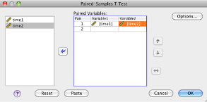
Click “OK.”
Look for the “Sig. (2-tailed)” column. This value is the \(p\) value.
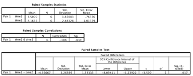
SPSS Output from a paired samples t-test
If \(p\) is less than .05, then you reject the null hypothesis (there is a significant difference between the groups) . If \(p\) is greater than or equal to .05, then you retain the null hypothesis (no conclusions can be made). Report the exact p value (for example, \(p\) = .017). A \(p\) value of .000 in SPSS just means that it was somewhere less than .001. Report a value of .000 as “\(p\) < .001.”
10.7.6 Conclude
If you reject the null, your conclusion matches your alternative hypothesis. If you retain, your conclusion is, “no conclusions can be made.”
10.7.7 Effect Size
When reporting results, you need to include the effect size. Mean difference is a measure of effect size that should always be included. Two other measures of effect size (choose one) are Cohen’s d and eta squared (η^2).
Cohen’s d is a measure of effect size for a t-test:
\({d}=\frac{\bar{X}_{difference}}{s_{difference}}\)
To find d, find the difference between each score, and calculate the mean and standard deviation of those differences. Use the sample statistic.
10.7.8 Interpretation of d (Cohen, 1988)
These are reference points, not firm cutoffs. For example, .45 is a medium effect size.
| Effect Size | Interpretation |
|---|---|
| \(d = \pm.2\) | Small effect |
| \(d = \pm.5\) | Medium effect |
| \(d = \pm.8\) | Large effect |
Eta squared (η^2) is yet another measure of effect size:
\(\eta^2=\frac{t^2}{t^2+n-1}\) Where n is the number of participants.
10.7.9 Interpretation of \(\eta^2\) and \(r^2\) (Cohen, 1988)
These are reference points, not firm cutoffs. For example, .056 is a medium effect size.
| Effect Size | Interpretation |
|---|---|
| \(\eta^2 = r^2 = .01\) | Small effect |
| \(\eta^2 = r^2 = .06\) | Medium effect |
| \(\eta^2 = r^2 = .14\) | Large effect |
10.7.10 Reporting your Results
Use this paragraph, changing the information to reflect your data:
A paired samples t-test was conducted to compare participants before and after receiving an experimental drug. There was a statistically significant increase in scores from time 1, before the drug was administered (M = 3.50, SD = 1.87), to time 2, after the drug was administered (M = 8.17, SD = 2.48), t(5) = -3.50, p = .017, 95% CI [-8.09, -1.24]. A large effect was observed, d = .71.
10.8 Reporting p-Values from SPSS
In your results paragraphs, you will need to report p-values. SPSS labels p-values “Sig.” In APA-style, report the exact p-value. Examples:
| SPSS Reports | Your results paragraph |
|---|---|
| Sig. = .032 | p = .032 |
| Sig. = .051 | p = .051 |
| Sig. = .731 | p = .731 |
There is one exception. If the \(p\)-value drops below .001, SPSS will cut off the trailing digits and show the value as “.000.” This is not zero! It is a number somewhere less than .001 (really, less than .0005 if you want to get technical). Report those as p < .001:
| SPSS Reports | Your results paragraph |
|---|---|
| Sig. = .000 | p < .001 |
The above example is the only time you should write p-values with anything except an equals sign. The “p < .05” notation is a throwback to the days before we had software to calculate exact p-values. A lot of information is contained in your statistical results, so it’s important to report them accurately.
10.9 APA Style Basics for Results Paragraphs
Spacing: Notice the single space on either side of the equals sign and less than sign. In APA style, you should leave a single space around every math operator (e.g., = > < + *) to improve readability.
Italics: Greek letters, subscripts, and superscripts are never italicized (e.g., ). All other statistical symbols should be italicized (e.g., M, p) when typing.
Leading zeros: Add a leading 0 for decimals only when the statistic can exceed 1. For example, write 0.19 cm but p = .19.
Rounding: There is no simple rule for rounding except that you should round numbers in manuscripts. When in doubt, round to two decimal places. p-values and effect size measures (d and \(\eta^2\)) should be reported to three decimal places.
10.10 Conducting an Independent Samples t-Test
10.10.1 Check Assumptions
- All assumptions of a paired samples t-test also apply to independent samples t-tests with one addition:
- Homogeneity of variance a.k.a. equality of variances a.k.a. homoscedasticity: Each group should have the same variance. You can check to see if you have violated this assumption using Levene’s test in SPSS.
10.10.2 Data Needed
To run an independent samples t-test, you need two variables. The first is a grouping variable. The grouping variable is a discrete, usually categorical variable that tells what group (example: experimental or control) the participant was in. Put another way: the grouping variable lists the level of your between-subjects independent variable for each participant.
10.10.3 Write Hypotheses
One-tailed version where it is expected that the first population mean will be larger than the second population mean (reverse the signs if it is expected that the sample mean will be smaller than the population mean):
\(H_0:\mu_1-\mu_2\leq0\)
in words: “the null hypothesis is that the mean of [name of sample 1] will be less than or equal to the mean [name of sample 2]”
\(H_a:\mu_1-\mu_2>0\)
in words: “the alternative hypothesis is that the mean of [name of sample 1] will be greater than the mean of [name of sample 2]” Two-tailed version:
\(H_0:\mu_1-\mu_2=0\)
in words: “the null hypothesis is that the mean of [name of sample 1] will equal the mean of [name of sample 2]”
\(H_a:\mu_1-\mu_2≠0\)
in words: “the alternative hypothesis is that the mean of [name of sample 1] will be different than the mean of [name of sample 2]”
10.10.4 Analyze & Decide – By Hand
This is an independent samples t-test.
\({t}=\frac{\bar{x_1}-\bar{x_2}}{\sigma_{\bar{X}}}\)
Standard error: \(\sigma_{\bar{X}}=\sqrt{\frac{s^2_1}{n_1} +\frac{s^2_2}{n_2}}\)
\(CI = \bar{X}\pm{t_{critical}} * \sigma_{\bar{X}}\)
\(df = n_1 + n_2 - 2\)
After computing t, find the critical value of t in the t-table. If t is beyond the critical value, then reject the null hypothesis. Otherwise, retain the null.
10.10.5 Analyze & Decide – Using SPSS
- Select “Independent-Samples T Test.”
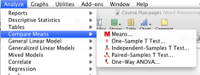
SPSS Analyze menu showing compare means selected
Move the dependent variable into the “Test Variable(s)” box. Move the grouping variable into the “grouping variable” box.
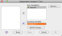
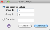
Click “Define groups” and then set the button to “Use specified values.” You have to tell SPSS what your coding scheme is for the grouping variable. In this example, our groups are “1” and “2.” Click “Continue.”
Click “OK.”
10.10.5.1 Levene’s Test for Equality of Variances
You check this after your test is run. Examine the output for Levene’s Test for Equality of Variances. If Sig. value is larger than .05, you have not violated the assumption. If Sig. value is less than .05, you have violated the assumption. If violated, use the “equal variances not assumed” line for all further interpretation. If not violated, use “equal variances assumed.”
Look for the “Sig. (2-tailed)” column (note: this is the one near the middle of the table–be careful so that you don’t accidentally use the Levine’s test Sig. value). Find the value of either “equal variances assumed” or “equal variances not assumed” according to your check of Levine’s test in the previous step. This value is the p value of your test.
If p is less than .05, then you reject the null hypothesis (there is a significant difference between the groups). If p is greater than or equal to .05, retain the null hypothesis (no conclusions can be made).
10.10.6 Conclude
If you reject the null, your conclusion matches your alternative hypothesis. If you retain, your conclusion is, “no conclusions can be made.”
An independent samples t-test was conducted to compare the effects of an experimental drug to no drug at all on anxiety scores. There was a statistically significant difference between the drug (M = 4.00, SD = 0) and no drug (M = 8.83, SD = 0.41) groups, t(5) = -29.00, p < .001, 95% CI [-5.26, -4.40]. Anxiety scores were higher in the no drug group. A large effect was observed, \(\eta^2\) = .99.
10.10.7 Effect Size
Mean difference is a measure of effect size. Another is eta squared (η^2). Eta squared (η^2) can be interpreted as “the proportion of variance accounted for.”
\(\eta^2=\frac{t^2}{t^2+n_1+n_2-2}\)
Where \(n_1\) is the number of participants in group 1 and \(n_2\) is the number of participants in group 2.
Review how to interpret \(\eta^2\), which is the same as \(r^2\)