Chapter 12 Regression

12.1 IVs and DVs

Remember the two things a true experiment must include: a manipulation and random assignment. Another way of describing this is that you must have some independent variable (IV) and some dependent variable/measure (DV). The IV is the variable “I control”; you, the experimenter, determines who or when participants are exposed to one level of the variable or another. Example IVs: experimental drug or placebo, new training or old training, no alcohol or one drink or two drinks, fast treadmill or slow treadmill or stationary treadmill. Your DV is what you measure, the thing that should change as a result of your manipulation. Example DVs: anxiety level, time to run a mile, lane crossings while driving, heart rate.

Recommended reading: A Brief explanation of IVs and DVs

12.2 The Regression Line

In correlation, we are looking for linear relationships. We have seen that these relationships have two components:

• Strength (the effect size). How strongly does one variable predict the other? On the graph: how well the dots hug the line. From r: values closer to +/-1 are stronger. Values closer to 0 are weaker.
• Direction (positive linear or negative linear). On the graph: does the line slope up (positive correlation) or slope down (negative correlation)? From r: positive values are positive correlations; negative values are negative correlations.

There is a third component: the line itself. The exact slope and the y-asymptote make one more thing possible: prediction. If you have a strong (i.e., significant) correlation, you make a good prediction of the value of one of the two variables if you know the value of the variable. So if smoking and diabetes are correlated, and I know whether or not someone smokes, I can make a good prediction about whether or not they have diabetes, and vice-versa. This line is called the regression line. To do this, we will use another analysis that is very similar to correlation, but our new analysis will also tell us what the line is, so that we can make predictions. This new analysis is called regression.

Regression aims to minimize the residuals for each score. A residual is the distance between each score and the regression line. The best regression line results in the smallest sum of squared residuals.

12.3 Finding the Regression Line

There are two steps to finding a regression line. First, compute b, which is the slope of the line:

\({b}=r(\frac{s_y}{s_x})\)

In words, b is equal to the value of r multiplied by the ratio of the standard deviations for the two variables.

The second step is to find the y-intercept. To find the y-intercept, use this equation:

\(a=\bar{y}-m{\bar{X}}\)

Now you can fill in the values of a and b to complete the regression equation:

\(\hat{y}=a+bx\)

With a complete regression equation, you can predict the value of y from any known value of x.

12.4 Simple Regression versus Multiple Regression

Using regression instead of correlation allows for us to increase the complexity. When we have two variables included (one IV and one DV), the result is called simple regression. Simple regression is the same statistical procedure as correlation. The only difference is the option selected in SPSS. We can, however, include more than one independent variable and use them collectively to predict a single dependent variable. For example, we can use smoking, diet, and exercise together to predict the risk for heart disease. When we throw multiple IVs into the analysis, we are performing multiple regression.

In multiple regression, all your IVs get combined to predict your DV.

Ultimately, we will be able to fully describe a line that best predicts the DVs from the combination of the IVs. The mathematical equation for a line is:

\(\hat{y}=a+bx\)

where y is the DV, x is the IV, b is the slope of the line, and a is the y-intercept (the height at which the line crosses the y axis).

Regression analysis, besides telling you the same things we found in correlation, will tell you the slope of the line (labeled b or beta) and the y-intercept.

12.5 The General Linear Model

If we re-write the equation of a line in this form, it describes a general linear model.

\(y = b_0 + b_1x_1 + e\)

\(y = b_0 + b_1x_1 + b_2x_2 + b_3x_3 ... + b_nx_n + e\)

where y is the DV (it stays as ‘y’), x is the single IV (it stays as ‘x’) or a combination of the IVs, b is the slope of the line (a number goes here), and b0 is the y-intercept (another number goes here). We have a new term here, e, which describes the error in the prediction. The e is theoretical; it represents the difference between your predicted DV and the real value of the DV. It is written as ‘e.’

12.6 The Regression Coefficients

b (‘B’ in SPSS): b is the unstandardized slope of the line. In other words: b is the expected change in the DV associated with 1 unit of change on the IV while holding the other variables constant. Each IV will have its own b value. The combination of all the b’s together is what makes the slope of the final line. In regression, b is a value like r which tells you strength (effect size) and direction. The difference is that b applies to a single IV while r applies to the entire regression model.

\(\beta\) (‘Beta’ in SPSS): Beta is the standardized slope of the line. Standardized means converted to z-scores. Beta scores are based on standardized IVs and DVs, but this makes them more complicated to interpret, and prone to fluctuations; avoid using them when comparing values across different regression models. However, the highest Beta score tells you which IV in your model had the strongest effect.

Confusing Symbol Alert: This is a completely different concept than ‘Beta’ in null hypothesis significance testing (NHST). In NHST, beta is the probability of committing a Type II error.

12.7 Regression - SPSS

12.7.1 Research Questions

How are one or more independent variables (IVs) related to a dependent variable (DV)?

The first step is to identify which variable is the DV and which variable(s) is/are the IV(s).

12.7.2 Check Assumptions

Level of measurement. You need:

• A continuous DV
• One or more continuous or dichotomous IV(s) (dichotomous variables are discrete variables that have only two values). Discrete variables may be used as IVs if they are dummy coded. This technique beyond the scope of this course as it must be done manually before running the analysis in SPSS. In this case, using some form of ANOVA may be easier.
• Independent observations. Each observation/case does not affect the measurement of any other observation/case.
• No outliers. You should generate a histogram for each of your variables to look for outliers. Outliers will typically reduce r. No multicollinearity . Multicollinearity occurs when your IVs are highly correlated with each other or with combinations of other IVs (r > .90 or r < -.90). Check the VIF (described below in the analyze step). If VIF is greater than 4, then you have multicollinearity and should consider excluding one of your IVs. Some authors argue that only VIF greater than 10 indicates multicollinearity. For this course, use 4 as the cutoff.
• No singularity . Singularity occurs when one IV is simply a calculation or combination of one or more other IVs. You can’t test for this in SPSS; you have to ask yourself if this is a problem with your data. We won’t emphasize this assumption in this course.

12.7.3 Write Hypotheses

You will have one pair of hypotheses for each IV. In a model with one DV and 2 IVs, you would have 4 total hypotheses (2 Ho and 2 Ha).

\(H_0: b_1 = 0\)

in words: the null hypothesis is that the regression coefficient for variable 1 will equal 0

\(H_a: b_1 \ne 0\)

in words: the alternative hypothesis is that the regression coefficient for variable 1 will not equal 0

\(H_0: b_2 = 0\)

in words: the null hypothesis is that the correlation coefficient for variable 2 will equal 0

\(H_a: b_2 \ne 0\)

in words: the alternative hypothesis is that the correlation coefficient for variable 2 will not equal 0

…and so on.

12.7.4 Analyze

Go to “Analyze” menu, then “Regression,” then “Linear.”

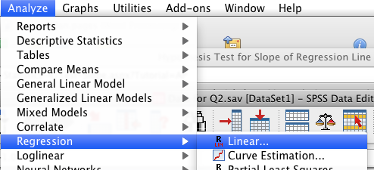
SPSS Analyze menu showing Regression and Linear selected

Click on your dependent variable (DV), then click the arrow to move it to the “Dependent” box. Click on your first independent variable (IV), then click the arrow to move it to the “Independent(s)” box. You can add as many IVs as you want in the “Independent(s)” box. Leave “Method” set to “Enter.”

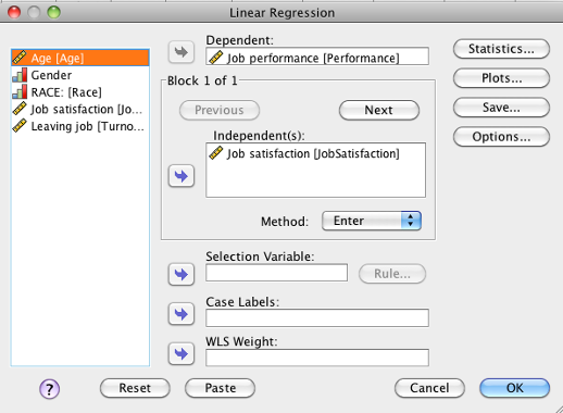
SPSS Linear Regression dialog box showing job performance as dependent and job satisfaction as independent

Click on the “Statistics” button. Check these boxes: “Estimates,” “Model fit,” “Descriptives,” and “Collinearity diagnostics” as shown below:

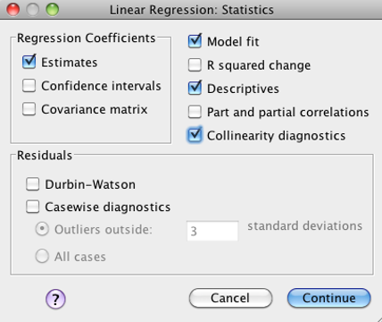
SPSS Linear regression statistics dialog box showing estimates, model fit, descriptives, and collinearity diagnostics

Click “Continue.” Then click either “OK” or “Paste” and go to your output window.

12.7.5 Decide

12.7.5.1 Check for Multicollinearity

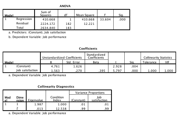
First, check your assumption of no multicollinearity. Look for the “Coefficients” table. Find the column “VIF.” You want to make sure that VIF is less than 4 for each one of your IVs. If VIF <= 4, you have not violated this assumption (great!). If VIF > 4, you have violated the assumption and should consider excluding one or more IVs from your model.

12.7.5.2 Evaluating the Entire Regression

Next, check the omnibus test. The omnibus test tells you if your entire regression model is statistically significant. Look at the “Sig.” column of the “ANOVA” table. You want to look at the “Sig.” value of “Regression.” If it is .050 or less, your entire regression is significant. If it is not significant, you retain all your null hypotheses and stop here.

In SPSS, “Sig.” is the value of p, the probability of obtaining these results if the null hypothesis were true.

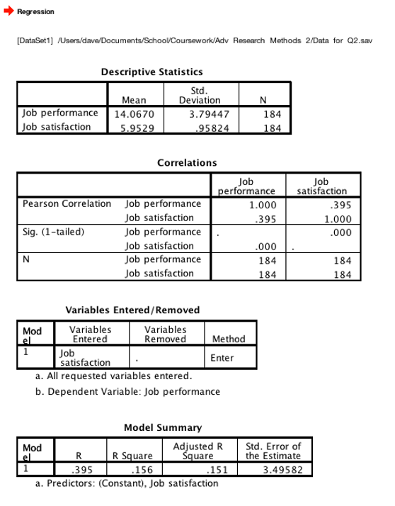
Once your model is statistically significant, you can find the r value in the “Model Summary” table. “Adjusted R Square” tells you the proportion of variance that your model accounts for. In this example, 15% of the variance is accounted for by the regression equation. Adjusted R Square of 1 would mean that the line perfectly predicts all the cases (100% of variance accounted for).

12.7.5.3 Evaluating Each IV

Once you know that your model is statistically significant, you can check each individual IV. Look for the “Sig.” column in the “Coefficients” table. Each IV that has a Sig value of .050 or less is significant, and you can reject the appropriate null hypothesis. Each IV also has a “B” value, which is that IVs contribution to the slope of the line. The y-intercept is the “B” value of “(Constant)”–in this case it is 4.761.

12.7.6 Conclude

12.7.6.1 Conclusions about the whole regression model

If you retained the null, there is no conclusion (and you can stop here). If you rejected the null, your conclusion is “the omnibus test for the regression was significant, p < .05, accounting for 15% of the variance.”

Remember, the proportion of variance accounted for is equal to the “Adjusted R Square” from the “Model Summary” table.

12.7.6.2 Conclusions about each IV

If you retained the null, there is no conclusion. If you rejected the null, your conclusion is that this IV predicts the DV. Depending on your design, you may say that this IV causes a change in the DV (experiment) or that the IV is related to the DV (quasi- and non-experiment).

This is the end of your conclusions. If you have a good regression equation, you can then make predictions:

12.7.6.3 Making predictions using the regression line

Finally, you can give the regression line:

\(y = b_1x_1 + b_2x_2 + b_3x_3 + b_4x_4 + b_{constant} + e\)

• where: \(b_1\) is the \(b\) value of IV #1
• \(b_2\) is the \(b\) value of IV #2, and so on
• \(b_{constant}\) is the \(b\) value of “(Constant).”

Using the example output, the equation would be:

\(y = 1.56x_1 + 4.76 + e\)

You can now predict other values using your equation. For example, if I know that my IV (job satisfaction) equals 6, I can predict the DV (job performance) using the equation:

\(y = 1.56 * 6 + 4.76\) (the \(e\) is theoretical and thus not part of the calculation), giving me a predicted DV of 14.12.

If your regression model is really strong (i.e., predicts a lot of variance/has a large R-squared), then creating this line lets you make some good predictions based on new data.

12.8 Results Paragraph

A multiple regression analysis was used to see if job satisfaction predicted job performance. The omnibus test for the regression was significant, accounting for 15.1% of the variance, F(1, 182) = 33.60, p < .001, \(R_{adj}^2\) = .151. Job satisfaction was a significant predictor, p < .001, b = 1.56, t(182) = 5.80. On average, people with higher job satisfaction had higher levels of job performance.

Where does this information come from?

• A multiple regression analysis was used to see if job satisfaction [and any other IVs] predicted job performance. Include the name of the analysis and list the independent and dependent variables.
• The omnibus test for the regression was significant, Did you reject the null for the entire model?
• accounting for 15.1% of the variance, Adjusted R square
• F(1, Degrees of freedom for the regression in the ANOVA table
• 182. Degrees of freedom for the residual in the ANOVA table
• = 33.60. The value of F for the regression in the ANOVA table.
• p < .001, From “Sig” in the ANOVA table
• \(r_{adj}^2\) = .151 Adjusted R square (really, this value only needs to be included once, but you should identify it as “adjusted R square”
• Job satisfaction was a significant predictor, p < .001, The first IV. You’ll have 8-12 for each IV. The p value comes from the “Sig” for this IV.
• b = 1.56, The unstandardized coefficient for this IV
• t(182) = Degrees of freedom for the residual in the ANOVA table
• 5.80. The value of t for this IV.
• On average, people with higher job satisfaction had higher levels of job performance. A plain-English interpretation of the relationship between this IV and the DV